5. The Kohn-Sham equation¶

Although we wish to solve the Schrodinger equation here:

\[\left(-\frac{\hbar^2\,\nabla^2}{2m} + V_{ext}({\bf r}) \right)\,\Psi({\bf r}) = E\,\Psi({\bf r})\]

where in Hydrogen actoms we pick \(V_{ext} = -\frac{e^2}{r}\). However once we move beyond one electron systems we find the system looking a little more complicated, there is a nucleus-electron attraction, electron-electron repulsion as well as electron spin considerations to add in also.

Although we know from solving the Hydrogen atom Schrodinger equation analytically, electrons get arranged into orbitals, e.g. Hydrogen has an electronic configuration \(1s^1\) and Carbon has an electronic configuration \(1s^2\,2s^2\,2p^2\). The use of orbital wavefunctions \(\phi({\bf r})\) allows us to simplify the picture to solve for l;larger and larger atoms with many electrons. This is known as the Hartree approximation and serves us well up to a point - it does not reflect the anti-symmetric nature of electrons (this is down to their spin). The adjustment we make to the system is to consider the Slater determinant:

\[\begin{split}\Psi({\bf r_1},s_1;\, {\bf r_2}, s_2;\,\dots) = \begin{vmatrix} \phi_1({\bf r_1},s_1) & \phi_1({\bf r_2},s_2) & \dots & \phi_1({\bf r_N},s_N) \\ \phi_2({\bf r_1},s_1) & \phi_2({\bf r_2},s_2) & \dots & \phi_2({\bf r_N},s_N) \\ \vdots & \vdots & \ddots & \vdots \\ \phi_N({\bf r_1},s_1) & \phi_N({\bf r_2},s_2) & \dots & \phi_N({\bf r_N},s_N) \ \end{vmatrix}\end{split}\]

The Hartree-Fock equation is essentially the Schrodinger equation for the ** orbital ** energy levels:

\[\left(-\frac{\hbar^2\,\nabla^2}{2m} + V_N({\bf r}) + V_H({\bf r}) + V_{x}^i({\bf r})\right)\,\phi_i({\bf r}) = \mathcal{E}_i\,\phi_i({\bf r})\]

wher \(V_x^i({\bf r})\) is an orbital dependent term.

The issue is that solving these one by one and then finding the total energy contriution thanks to every electron is very time consuming and computational impractical, thus we need to simplify.

We attempt to use an electron density field \(\rho({\bf r})\) here to help solve these equations, this has the advantage of not treating the electgrons as separate entities, but rather as one large field that we can attempt to find - hence we will drop the individualk orbital exchange terms for one large overall exchange term \(V_x^i \rightarrow V_{XC}\). Another assumption is to think about only the outer electrons as the relevent ones, those in filled electrong shells (so called tight binding) do not really play a big role in the energies of outer electrons.

The nuclear potential is the easiest term to consider:

\[\]

The electron charge density can be found as:

\[\rho({\bf r}) = e\,\sum_{i,\,occuped}^N |\phi_i({\bf r})|^2 = \sum_n f_n|\phi(r)|^2\]

where \(f_n\) is the occupation number of the electrons in each orbital. When we have an even number of electrons in the atom, each orbital is fully filled so \(f_n = 2\), whereas for an odd number there will be a partially filled orbital somewhere, so \(f_n = 1\).

Our Hatree potential term can be found from electromagnetism (Gauss’s law in potentials):

\[\nabla^2 V_H({\bf r}) = -4\pi e\,\rho({\bf r})\]

This can be solve for \(V_H\) using a greens function:

\[V_H = \iiint \frac{e^2\,\rho({\bf r})}{|{\bf r - r'}|}\,\mathrm{d}^3r' = e^2\int_0^{\infty}\frac{\rho({\bf r})}{|r - r'|}\,\mathrm{d}r'\]

One problem with solving this in one dimension is that it won’t converge - there will be a some sort of divergence in each of the terms, so we modify this expression slightly:

\[V_H = e^2\int_0^{\infty}\frac{\rho({\bf r})}{\sqrt{(r - r')^2+\epsilon}}\,\mathrm{d}r'\]

by adding in a term \(\epsilon < 1\). This term is just here for numerical stability, it aboids infinities where we least want them.

In atomic units, this looks like:

\[V_H = \int_0^{\infty}\frac{\rho({\bf r})}{\sqrt{(r - r')^2+\epsilon}}\]

After we applied the local density approximation, the exchange term actually looks like:

\[V_{XC} = -\left(\frac{3\,\rho}{\pi}\right)^{1/3}\]

this is nice and simple, before the approximation this expression would look VERY complicated.

This leads us to the Kohn-Sham (KS) equations:

\[\left(-\frac{\hbar^2}{2m} \nabla^2 + V_N + V_H + V_{xc}\right)\,\phi_i = \mathcal{E}_i\,\phi_i\]

We aim to solve this system iteratively:

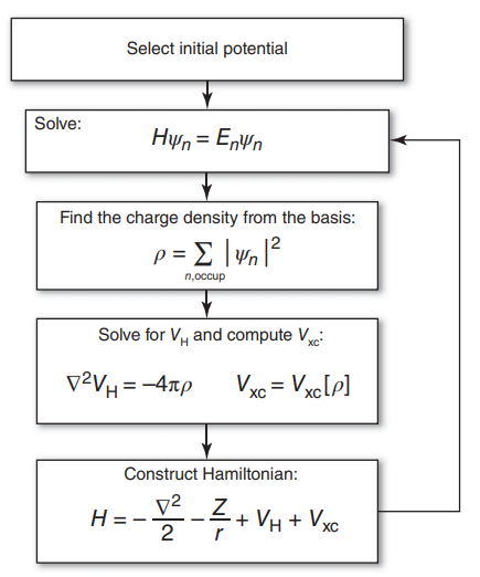
Fig. 5.1 A schematic for following the self-consistent field approach to solve the KS equations.¶

We call this the self-consistent field approach to solve the KS equations, where we iteratively solve this system to find energies and wavefunctions.

If we use the KS to calculate the system initially, then reformulate the Hamiltonian operator here using the

One we have solutions from the system, we can also calculate the different parts of the energy contribution:

\[\begin{split}E_H &= \frac{1}{2}\iint \frac{\rho(r)\,\rho(r')}{|r-r'|}\,\mathrm{d}r\,\mathrm{d}r' \\ E_{XC} &= -\frac{3^{4/3}}{\pi^{1/3}}\,\int (\rho(r))^{4/3}\,\mathrm{d}r\end{split}\]

Density Functional Theory

The Kohn-Sham equation

5. The Kohn-Sham equation¶