1. Integration

1.1. Arc Length

Suppose that we have a function \(y = f(x)\), we know through integration that we can find the area under the curve:

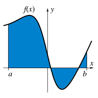
Fig. 1.1 The area (in blue) under a function \(f(x)\) over the interval \(x \in [a,\,b]\) given by the integral \(\displaystyle \int_a^bf(x)\,\mathrm(d)x\).

Another question that we could ask however is what is the length of the path traced out by the function \(f(x)\) over the range \([a,\,b]\):

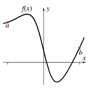
Fig. 1.2 The path traced out by the function \(f(x)\) over the interval \(x \in [a,\,b]\).

To find an expression for this length \(S\), we can break up the path into infinitesimal segments and then integrate these over the whole function. We can see this process breaking down the change in arc length \(\Delta s\) by Pythagoras graphically as:

\[(\Delta s)^2 = (\Delta x)^2 + (\Delta y)^2 \Rightarrow \Delta s = \sqrt{(\Delta x)^2 + (\Delta y)^2} = \Delta x\,\sqrt{1 + \left(\frac{\Delta y}{\Delta x}\right)^2}\]

Fig. 1.3 Left Pane: Breaking down path legnth segment \(\Delta s\) into \(x,\, y\) components \(\Delta x,\, \Delta y\). The distance \(\Delta s\) moved along a curve, corresponding to small changes \(\Delta x \Delta y\) can be calculated by Pythagoras’ formula.

Right Pane: Effect of taking the limit of smaller \(\Delta x\) in finding the path length. By decreasing the difference \(\Delta x\) between the joined up points, we obtain a better approximation.

Taking the limit of \(\Delta x\rightarrow 0\) we find:

\[\mathrm{d}s = \mathrm{d}x\, \sqrt{1 + \left(\frac{\mathrm{d}y}{\mathrm{d}x}\right)^2}\]

and therefore to find the path length:

\[L = \int_{x=a}^{x=b} \mathrm{d}s = \int_a^b \sqrt{1 + \left(\frac{\mathrm{d}y}{\mathrm{d}x}\right)^2}\,\mathrm{d}x\]

We might also have a function which is parameterised \(y = y(t),\, x=x(t)\), it is also possible to find an expression for the path length for \(t \in [t_a,\, t_b]\), taking the limit of \(\Delta t \rightarrow 0\):

\[\begin{split}\Delta s &= \Delta t\,\sqrt{\left(\frac{\Delta x}{\Delta t}\right)^2 + \left(\frac{\Delta y}{\Delta t}\right)^2} \\ \Rightarrow \mathrm{d}s &= \mathrm{d}t\, \sqrt{\left(\frac{\mathrm{d}x}{\mathrm{d}t}\right)^2 + \left(\frac{\mathrm{d}y}{\mathrm{d}t}\right)^2}\\ L &= \int_{t_a}^{t_b} \sqrt{\left(\frac{\mathrm{d}x}{\mathrm{d}t}\right)^2 + \left(\frac{\mathrm{d}y}{\mathrm{d}t}\right)^2}\,\mathrm{d}t\end{split}\]

Worked examples

1. Looking at \(y = \cosh(x)\) over the range \(x \in [0,\,1]\), so we find \(\mathrm{d}y/\mathrm{d}x = \sinh(x)\), and therefore:

\[L = \int_0^1 \sqrt{1 + \sinh^2(x)}\,\mathrm{d}x = \int_0^1 \cosh(x)\,\mathrm{d}x = \Big[ \sinh(x) \Big]_0^1 = \sinh(1) \simeq 1.175\dots\]

2. Consider a circle, parameterised by \(x = R\cos(t),\, y = R\sin(t)\), over the range \(t \in [0,\, 2\pi)\), giving \(\mathrm{d}x/\mathrm{d}t = -R\sin(t),\, \mathrm{d}y/\mathrm{d}t = R\cos(t)\) and therefore:

\[L = \int_0^{2\pi} \sqrt{R^2\sin^2(t) + R^2\cos^2(t)}\,\mathrm{d}t = \int_0^{2\pi} R\,\mathrm{d}x = \Big[ Rt \Big]_0^{2\pi} = 2\pi\,R\]

which gives the result for the circumference of a circle!

Practice questions

1. Find the length of the arc of the curve \(x = 18t^2\), \(y=(12t+9)^\frac{3}{2}\) from \((0,27)\) to \((32, 125)\).

2. Calculate the arc length of the curve defined by \(x=\cos(t)\), \(y=\sin(t)\), between \(t=\frac{\pi}{6}\) and \(t=\frac{\pi}{3}\).

3. Calculate the length of the curve \(y=2(x-1)^\frac{3}{2}\) between \(x=1\) and \(x=4\).

Solutions

1. Find the length of the arc of the curve \(x = 18t^2\), \(y=(12t+9)^\frac{3}{2}\) from \((0,27)\) to \((32, 125)\).

We have:

\[\frac{\mathrm{d}x}{\mathrm{d}t}=36t, \quad \frac{\mathrm{d}y}{\mathrm{d}t}=\frac{3}{2} (12)(12t+9)^{1/2}=18(12t+9)^{1/2}\]

Then, as all the lengths are positive:

\[L = \int_{t=0}^{4/3}\sqrt{(36t)^2+18^2(12t+9)}\mathrm{d}t = 18\int_{0}^{4/3}\sqrt{(3+2t)^2}\mathrm{d}t = 18\displaystyle \int_0^{4/3}(2t+3)\mathrm{d}t\]

Thus \(\displaystyle L=18\biggr[t^2+3t\biggr]_0^{4/3}=104\) units

2.

Calculate the arc length of the curve defined by \(x=\cos(t)\), \(y=\sin(t)\), between \(t=\frac{\pi}{6}\) and \(t=\frac{\pi}{3}\).

\[\int_{\pi/6}^{\pi/3}\sqrt{\left(\frac{\mathrm{d}x}{\mathrm{d}t}\right)^2+\left(\frac{\mathrm{d}y}{\mathrm{d}t}\right)^2}\mathrm{d}t =\int_{\pi/6}^{\pi/3}\sqrt{\sin^2(t)+\cos^2(t)}\mathrm{d}t =\left[t\right]_{\pi/6}^{\pi/3}=\frac{\pi}{6}\]

The result simply gives the arc length of a portion of the unit circle (\(x^2 + y^2 = 1\)) between \(\theta=\frac{\pi}{6}\) and \(\theta=\frac{\pi}{3}\)

3.

Calculate the length of the curve \(y=2(x-1)^\frac{3}{2}\) between \(x=1\) and \(x=4\).

\[\frac{\mathrm{d}y}{\mathrm{d}x}=3\sqrt{x-1}, \quad \mathrm{d}S = \sqrt{1+\left(\frac{\mathrm{d}y}{\mathrm{d}x}\right)^2}\,\mathrm{d}x=\sqrt{1+9(x-1)}\,\mathrm{d}x=\sqrt{9x-8}\,\mathrm{d}x\]

and therefore:

\[S= \int_{x=1}^{x=4}\sqrt{9x-8}\,\mathrm{d}x = \int_1^4(9x-8)^{1/2}\,\mathrm{d}x = \left[\frac{2}{27}(9x-8)^{3/2}\right]_1^4 = \frac{2}{27}(56\sqrt{7}-1)\]

1.2. Surfaces of Revolution

Lets now go further, what happens if we take a function and rotate it around an axis:

Fig. 1.4 Left Pane: Rotating a function \(y = f(x)\) around the \(x\) axis, over \(x \in [a,\, b]\) producing a solid of revolution, Right Pane: Breaking down the volume into discrete slices, each of width \(\mathrm{d} x\).

To find the volume of such a rotated solid, we need to think about the cross sectional area along the range, which will be \(\pi \,y^2\) since the radius of each slice at \(x\) is \(y(x)\). Then we just need to integrate up these slices \(\pi\,y^2\,\mathrm{d}x\) over the range:

\[V_x = \int_a^b \pi\,y^2\,\mathrm{d}x\]

and we can swap round the axis we rotate over to the \(y\) axis and therefore the radius of each slice would be \(\pi\,x^2\) and therefore:

\[V_y = \int_{y(a)}^{y(b)} \pi\,x^2\,\mathrm{d}y\]

Note

Instead of using cylindrical slices, we could use “frustrums” (sections of cones). The result would be the same (in the limit \(\Delta x \rightarrow 0\)).

Similarly, when calculating the area under the curve, we used rectangles, but we could have used parallelograms.

We can also find the surface area of this solid of revolution, if we rotate over the \(x\) xcis then this surface area is the circumference of each slice \(2\pi\,y\) multiplied by the path length \(\mathrm{d} s\) along the surface, so we find:

\[A_x = \int_{x=a}^{x=b} 2\pi\,y\,\mathrm{d}s = \int_a^b 2\pi\,y\,\sqrt{1 + \left(\frac{\mathrm{d}y}{\mathrm{d}x}\right)^2}\,\mathrm{d}x\]

We could rotate over the \(y\) axis instead, in which case we just switch the circumference we are interested in to be \(2\pi\,x\) and integrate the path length over the \(y\) axis:

\[A_y = \int_{y(a)}^{y(b)} 2\pi\,x\,\mathrm{d}s = \int_{y(a)}^{y(b)} 2\pi\,x\,\sqrt{1 + \left(\frac{\mathrm{d}x}{\mathrm{d}y}\right)^2}\,\mathrm{d}y\]

Worked example

Lets find the volume of a cone depicted in Fig. 1.5, with height \(h\) and circular radius \(R\), so \(y = R x / h\) over the range \(x \in [0,\, h]\):

\[\begin{split}V_x = \int_0^h \pi\,\left(\frac{R x}{h}\right)^2\,\mathrm{d}x = \frac{R^2 \,\pi}{h^2}\Big[ \frac{1}{3}x^3\Big]_0^h = \frac{1}{3}\pi \,R^2\,h\\\end{split}\]

which matches the expression we expect and explains where this factor of \(1/3\) comes from!

Likewise we can look at the surface area of this cone, \(y = R x / h \rightarrow \mathrm{d}y/\mathrm{d}x = R / h\) over the range \(x \in [0,\, h]\):

\[\begin{split}A_x &= \int_0^h 2\pi\,\frac{R x}{h}\,\sqrt{1 + \left(\frac{R}{h}\right)^2}\,\mathrm{d}x \\ &= 2\pi \frac{R}{h}\sqrt{1 + \left(\frac{R}{h}\right)^2}\Bigg[ \frac{1}{2}x^2\Bigg]_0^h \\ &= \pi R h\sqrt{1 + \left(\frac{R}{h}\right)^2} = \pi R\sqrt{h^2 + R^2}\end{split}\]

where \(\sqrt{h^2 + R^2}\) is the slant length.

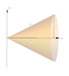
Fig. 1.5 Depiction of a function \(y = R x / h\) and the solid of revolution around the \(x\) axis - a cone.

Likewise if we have parametrised expressions \(x = x(t),\, y = y(t)\), over the range \(t \in [t_1,\, t_2]\) then these expressions become:

\[\begin{split}V_x &= \int_{t_1}^{t_2} \pi\,y^2\,\frac{\mathrm{d}x}{\mathrm{d}t}\,\mathrm{d}t \\ V_y &= \int_{t_1}^{t_2} \pi\,x^2\,\frac{\mathrm{d}y}{\mathrm{d}t}\,\mathrm{d}t \\ A_x &= \int_{t_1}^{t_2} 2\pi\,y\,\sqrt{\left(\frac{\mathrm{d}x}{\mathrm{d}t}\right)^2 + \left(\frac{\mathrm{d}y}{\mathrm{d}t}\right)^2}\,\mathrm{d}t \\ A_y &= \int_{t_1}^{t_2} 2\pi\,x\,\sqrt{\left(\frac{\mathrm{d}x}{\mathrm{d}t}\right)^2 + \left(\frac{\mathrm{d}y}{\mathrm{d}t}\right)^2}\,\mathrm{d}t\end{split}\]

Practice questions

1. Find the surface area of revolution for \(y = x^2\) rotated around the \(y\) axis over \(y \in [0,\,4]\).

2. Determine the surface area of the solid obtained by rotating the function \(y=\sqrt{9-x^2}\) for \(-2 \leq x \leq 2\) about the \(x\)-axis.

3. Determine the surface area of the solid obtained by rotating the function \(y=x^{1/3}\), for \(1 \leq y \leq 2\) about the \(y\)-axis.

4. Find the surface area spherical section obtained by revolving the function \(r = \cos(\theta)\) around the \(x\) axis over \(\theta \in \left[0\,\frac{\pi}{4}\right]\).

5. Find the volume of revolutio for the section obtained by reolving the function \(y = x^2\) around the \(x\) axis over \(x \in [-2,\,3]\).

6. Find the volume of the solid obtained by rotating the region bounded by \(y=2x^2\) and \(y=x^3\) about the \(x\) axis, from the origin up to where the functions meet.

Solution

1.

\[\begin{split}y = x^2\Rightarrow x = y^{1/2}\\ \frac{\mathrm{d}x}{\mathrm{d}y} = \frac{1}{2}y^{-1/2}\\ 1 + (x')^2 = 1 + \frac{1}{4}y^{-1} = \frac{1+4y}{4y}\end{split}\]

so integral is:

\[\begin{split}A &= \int_{y=0}^{y=4} 2\pi\,x\,\mathrm{d}s = 1\pi\int_0^4 x\,(1+4x^2)^{1/2}\,\mathrm{d}x \\ &= \frac{\pi}{4}\bigg[\frac{2}{3} (1+4x^2)^{3/2} \bigg]_0^2 = \frac{\pi}{6}\left(17^{3/2}-1\right) \approx 36.2\dots\end{split}\]

2.

\[\begin{split}y^2 &= 9-x^2\\ 2y\frac{\mathrm{d}y}{\mathrm{d}x} &= -2x \Rightarrow \frac{\mathrm{d}y}{\mathrm{d}x} = -\frac{x}{y} = -\frac{x}{\sqrt{9-x^2}}\\ 1 + \left( \frac{\mathrm{d}y}{\mathrm{d}x}\right)^2 &= 1 + \frac{x}{9-x^2} = \frac{9}{9-x^2}\end{split}\]

so integral is:

\[2\pi\,\int_{-2}^2 y\sqrt{1 + \left( \frac{\mathrm{d}y}{\mathrm{d}x}\right)^2}\,\mathrm{d}x = 6\pi\,\int_{-2}^2 \, \mathrm{d}x = 24\pi\]

3.

\[\begin{split}y &= x^{1/3} \Rightarrow x = y^3\\ \frac{\mathrm{d}x}{\mathrm{d}y} &= 3y^2 \\ 1 + \left( \frac{\mathrm{d}x}{\mathrm{d}y}\right)^2 &= 1+ 9y^4 \end{split}\]

the limits as \(y \in [1,\, 2]\), so integral is:

\[2\pi\,\int_{1}^2 x\sqrt{1 + \left( \frac{\mathrm{d}x}{\mathrm{d}y}\right)^2}\,\mathrm{d}x = 2\pi\int_{1}^2 y^3\left(1+9y^4\right)^{1/2}\, \mathrm{d}x\]

which we can solve by inspection (or reverse chain rule), where \(\int f^n\,f'\,\mathrm{d}y = \frac{1}{n+1}f^{n+1}\), here \(f = 1+9y^4 \), so \(f' = 36y^3\)

\[S = 2\pi\frac{1}{36}\Big[\frac{2}{3}\left(9y^4+1 \right)^{3/2}\Big]_1^2 = \frac{\pi}{27}\left(145^{3/2} - 10^{3/2} \right) \simeq 199.48\dots\]

4. Given that the surface for a rotated solid around the \(x\) axis is \(\int_a^b 2\pi y\,\mathrm{d}s\) and we have \(x = r \cos(\theta),\, y = r \sin(\theta)\), then this is just a parametric problem, where:

\[\begin{split}\mathrm{d}s &= \sqrt{\left(\frac{\mathrm{d}x}{\mathrm{d}\theta}\right)^2 + \left(\frac{\mathrm{d}y}{\mathrm{d}\theta}\right)^2}\,\mathrm{d}\theta\\ \mathrm{d}x &= \cos(\theta)\,\mathrm{d}r - r \sin(\theta)\,\mathrm{d}\theta \Rightarrow \frac{\mathrm{d}x}{\mathrm{d}\theta} = \cos(\theta)\,\frac{\mathrm{d}r}{\mathrm{d}\theta} - r \sin(\theta)\\ \mathrm{d}y &= \sin(\theta)\,\mathrm{d}r + r \cos(\theta)\,\mathrm{d}\theta \Rightarrow \frac{\mathrm{d}y}{\mathrm{d}\theta} = \sin(\theta)\,\frac{\mathrm{d}r}{\mathrm{d}\theta} + r \cos(\theta)\\ \mathrm{d}s &= \sqrt{r^2 + \left(\frac{\mathrm{d}r}{\mathrm{d}\theta}\right)^2}\,\mathrm{d}\theta \end{split}\]

Given that \(r = \cos(\theta)\) then:

\[\frac{\mathrm{d}r}{\mathrm{d}\theta} = -\sin(\theta)\]

so the problem looks like:

\[\begin{split}A &= \int_0^{\pi/4} 2\pi r\,\sin(\theta)\,\sqrt{\cos^2(\theta) + \sin^2(\theta)}\,\mathrm{d}\theta \\ &= \int_0^{\pi/4} 2\pi \cos(\theta)\,\sin(\theta)\,\mathrm{d}\theta = \Bigg[\pi \sin^2(\theta) \Bigg]_0^{\pi/4} = \frac{\pi}{2}\end{split}\]

5.

Using \(V = \int_{-2}^3 \pi y^2\,\mathrm{d}x \), we find:

\[V = \int_{-2}^3 \pi x^4\,\mathrm{d}x = \Bigg[ \frac{1}{5}x^5\Bigg]_{-2}^3 = \pi\left[ \frac{243}{5} - \left(-\frac{32}{5}\right)\right] = 55\pi\]

6.

Firstly lets find the intersection points:

\[\begin{split}x^3 &= 2x^2 \\ x^2(x-2) &= 0 \\ \Rightarrow x = 0,\qquad & x = 2\end{split}\]

which we can also see graphically:

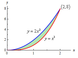
To find the volume of the bounded shape, we need to subtract the two volumes we would find:

\[\begin{split}V_{tot} &= V_{outer} - V_{inner} = \int_0^2 \pi (2x^2)^2 \,\mathrm{d}x - \int_0^2 \pi (x^3)^2 \,\mathrm{d}x \\ &=\int_0^2 \pi \left(4x^4 -x^6\right)\, \mathrm{d}x = \Bigg[ \frac{4}{5}x^5 - \frac{1}{7}x^7\Bigg]_0^2 = \frac{256}{35}\pi\end{split}\]