20. Faraday’s Law
Our discussion of both the Biot-Savart and Ampère’s laws tells us that moving charges (currents) produce magnetic fields. Since these currents are pushed by potential difference - driven by electric fields, these result in a magnetic field. The next question is can we start with a magnetic field and finish with an electric field - Faraday’s law tells us yes!
Thinking again about the link between moving charges and magnetic fields:
As we mentioned previously, we can think of \(Q\,{\bf v}\) is a current momentum, therefore taking the time derivative should produce a current force:
and we call this the electromotive force (EMF), denoted by \(\mathcal{E}\).
One potential question here is, as we saw in Fig. 17.8, an element of current carrying wire \(I\,\mathrm{\bf d} \ell\) produces a whole plane of magnetic field. Therefore to calculate the total contribution to the EMF, we need to find the magnetic flux \(\Phi_B\), giving us the form of Faraday’s law:
If we have a coil of wire, with \(N\) turns of wire, each of which cuts through magnetic field lines, as we see in Fig. 20.1. Faraday’s law applies to each turn, it acts like a series circuit across the field and so the EMF induced becomes an additive process, and so we have:
Note that the two sides of Equation (20.1) differ by a sign, this is known as Lenz’s law. This is here to ensure that we do not violate conservation of energy - the direction of an induced current which is pushed by the EMF \(\mathcal{E}\) is always such as to oppose the change in the magnetic field that produces it. This means that if we push a permanent magnet into a coil of wire, as we see in Fig. 20.1, the EMF which will push a current such that the magnetic field that Amp`eres law predicts would be created will oppose the magnetic field of the permanent magnet. If the current flowed in then opposite direction, it would cause the magnet to be dragged into coil faster and faster, creating a flow of limitless energy (which is clearly impossible).
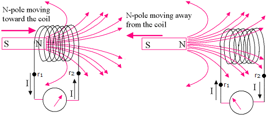
Fig. 20.1 Direction of induced EMF from a moving magnetic into a coil, Left - North pole moving into coil, Right - North pole moving out of coil.
20.1. Electrical Transformers
We can apply Faraday’s law to investigate the flow of magnetic fields and EMF’s in a transformer, as depicted in Fig. 20.2, where an initial voltage \(V_p\) typically pushes an initially large current \(I_p\) in the primary circuit and through the primary coil.
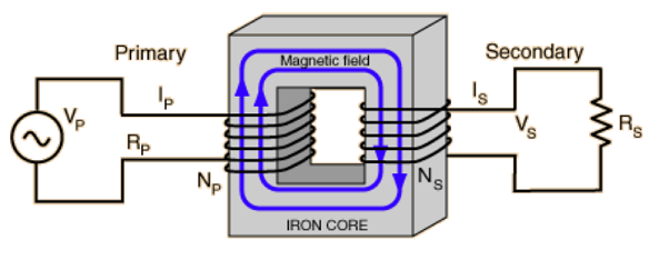
Fig. 20.2 Flow of magnetic flux in a transformer - we denote the left hand coil the Primary and right hand coil the Secondary, each carries a current \(I_{p,s}\) and EMF \(V_{p,s}\).
The alternating voltage in the primary circuit, say:
with some ohmic resistance \(R_p\), which pushes a current
through the primary coil. The total input energy in the primary coil therefore is:
and this is related to the output energy \(P_{out} = V_s\,I_s\), with \(P_{in} = P_{out}\). By Ampère’s law, we can see the time varying current creates a time varying magnetic field \(\Phi_B(t)\) in the primary coil. Then by Faraday’s law, the changing flux is related to the induced EMF \(\mathcal{E}\) in each coil as:
Since the magnetic flux moves through the iron core (and ignoring any losses), then we can combine the equations to find:
where \(a\) is the so called turns ratio. Combining with the energy conservation condition \(V_p\,I_p = V_s\,I_s\), we find different situations based on ratios of \(N_p,\,N_s\):