.md .pdf

repository open issue

Contents

4. Longitudinal Waves

4.1. Derivation from masses and springs

Lets start with the classic derivation of waves propagating, with a collection of \(N\) masses \(m\) connected together on springs (with spring constant \(k\)), each with equilibrium separation \(h\), as shown in Fig. 4.1. We can measure the horizontal displacement \(u(x,t)\) from the equilibrium positions.

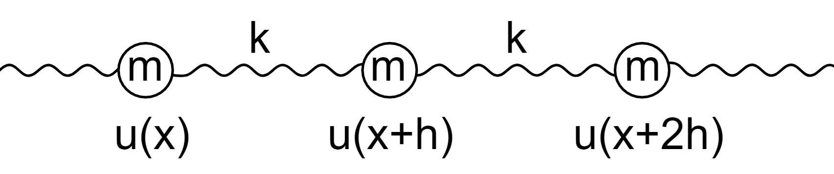
Fig. 4.1 Identical masses connected by identical springs.

If the springs follow Hooke’s law, then \(F_{H} = k\,u(x,t) \) and equally all the masses will follow Newton’s second law \(F_{N} = m \,a(x,t)\). We can analyse the dynamics of the middle mass, where the Hooke’s law forces will from both the spring \(x+h \rightarrow x+2h\) as well as the spring \(x \rightarrow x+h\)

\[\begin{split}F_N &= m \frac{\partial^2}{\partial t^2}u(x+h,t)\\ F_H &= k[u(x+2h,t) - u(x+h,t)] - k[u(x+h,t) - u(x,t)] \\ &= k[u(x+2h,t) - 2u(x+h,t) + u(x,t)]\end{split}\]

Since these defintions are equal, then by rearrangement:

(4.1)\[\frac{\partial^2}{\partial t^2}u(x+h,t) = \frac{k}{m}[u(x+2h,t) - 2u(x+h,t) + u(x,t)] \]

Lets also consider a chain of springs in series, as shown in Fig. 4.2

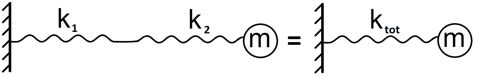
Fig. 4.2 Two springs in series with a mass

We can consider the total displacement of the mass \(m\), as well as as the individual springs displacements

\[\begin{split}F_{tot} &= k_{tot}\,x_{tot}\\ F_1 &= k_1\,x_1\\ F_2 &= k_2\,x_2\end{split}\]

If \(x_{tot}\) can be broken up into the individual springs displacements \(x_{tot} = x_1 + x_2\) then we simplify to:

\[F_{tot} = k_{tot}(x_1 + x_2)\]

by rearrangement this reduces to

\[\frac{F_{tot}}{k_{tot}} = \left(\frac{F_1}{k_1} + \frac{F_2}{k_2}\right)\]

Since the springs propagate the force applied through them, all the forces are the same \(F_{tot} = F_1 = F_2\), so we are finally left with:

\[\frac{1}{k_{tot}} = \frac{1}{k_1} + \frac{1}{k_2}\]

and therefore for two springs, the effective spring constant is:

\[k_{tot} = \left(\frac{1}{k_1} + \frac{1}{k_2}\right)^{-1}\]

If there are \(N\) springs in series, then this result takes the form:

\[\frac{1}{k_{tot}} = \frac{1}{k_1} + \frac{1}{k_2} + \dots + \frac{1}{k_N}\]

and if the springs are identical, \(k_1 = k_2 = \dots = k_N = k\) this result reduces to:

(4.2)\[\frac{1}{k_{tot}} = \frac{N}{k} \Rightarrow k_{tot} = \frac{k}{N}\]

We can substitute (4.2) into Equation (4.1):

\[\frac{\partial^2}{\partial t^2}u(x+h,t) = \frac{N\,k_{tot}}{m} [u(x+2h,t) - 2u(x+h,t) + u(x,t)]\]

Now if we want to consider the whole chain of masses and springs, then with \(N\) masses and total mass on the chain is \(m_{tot} = Nm\), which results in

\[\frac{\partial^2}{\partial t^2}u(x+h,t) = \frac{N^2\,k_{tot}}{m_{tot}} [u(x+2h,t) - 2u(x+h,t) + u(x,t)]\]

and if the the total chain length is \(L = Nh\), then:

(4.3)\[\Rightarrow \frac{\partial^2}{\partial t^2}u(x+h,t) = \frac{L^2\,k_{tot}}{m_{tot}} \frac{u(x+2h,t) - 2u(x+h,t) + u(x,t)}{h^2} \]

By taking the limit \(N \rightarrow \infty\) and therefore \(h \rightarrow 0\) for a finite chain length \(L\), this has exactly the form of the partial derivative in Equation (2.2). Hence Equation (4.3) has the form:

\[\frac{\partial^2}{\partial t^2}u(x+h,t) = \frac{L^2\,k_{tot}}{m_{tot}} \frac{\partial^2}{\partial x^2} u(x+h,t)\]

If we examine the units of the constants here:

\[\frac{[L]^2\,[k]}{[m]} = \frac{m^2\,N\,m^{-1}}{kg} = \frac{m\,kg\,m\,s^{-2}}{kg} = m^2\,s^{-2} = [speed]^2\]

This results in the well known form of the wave equation in one dimension:

(4.4)\[\frac{\partial^2 u}{\partial t^2} = c^2 \frac{\partial^2 u}{\partial x^2} \]

where \(c\) is the wave speed of some form (more on this later).

4.2. Longitundinal Wave Energy and Power

Given that waves are a method of propogating energy, it is an important question to ask how much and what parameters does a waves energy depend on!

Lets look at the total energy \(E\):

\[E = KE + PE\]

where \(KE\) is the total kinetic energy and \(PE\) the total potential energy.

Gping back to the masses and springs model, the potential energy of each mass shown in Fig. 4.1 would be:

\[PE = \dots + \frac{1}{2}k\Big[u(x+h,t) - u(x,t)\Big]^2 + \frac{1}{2}k\Big[u(x+2h,t) - u(x+h,t)\Big]^2 + \dots\]

where each of the springs in the chain will contribute to the PE of two masses, depending on their orientation. Notice here that there are not any terms like \(PE \sim \frac{1}{2}k u^2(x,t)\), this is because we haven’t considered the effects at either end of the chain - although these edge effects are really important in real world systems, we will omit them here.

Using the springs in series result from (4.2), we can rewrite the PE in the form:

\[PE = \frac{1}{2}\,N\,k_{tot} \left(\dots + \Big[u(x+h,t) - u(x,t)\Big]^2 + \Big[u(x+2h,t) - u(x+h,t)\Big]^2 + \dots \right)\]

and likewise if we introduce the size of the mass \(m\) and then consider the total chain mass:

\[\begin{split}PE &= \frac{1}{2}\frac{N\,k_{tot}\,m}{m}\left(\dots + \Big[u(x+h,t) - u(x,t)\Big]^2 + \Big[u(x+2h,t) - u(x+h,t)\Big]^2 + \dots \right) \\ &= \frac{1}{2}\,m\frac{N^2\,k_{tot}}{m_{tot}}\left(\dots + \Big[u(x+h,t) - u(x,t)\Big]^2 + \Big[u(x+2h,t) - u(x+h,t)\Big]^2 + \dots \right)\end{split}\]

and then looking at the total chain length \(L = N\,h\):

\[PE = \frac{1}{2}\,m\,\frac{L^2\,k_{tot}}{m_{tot} h^2}\left(\dots + \Big[u(x+h,t) - u(x,t)\Big]^2 + \Big[u(x+2h,t) - u(x+h,t)\Big]^2 + \dots \right)\]

We recongise the term \(c^2 = L^2\,k_{tot}/m_{tot}\) and as before by taking the limit of \(N \rightarrow \infty \Rightarrow h \rightarrow 0\):

\[PE = \frac{1}{2}\,m\,c^2\,\lim_{h \rightarrow 0}\left(\dots + \Big[\frac{u(x+h,t) - u(x,t)}{h}\Big]^2 + \Big[\frac{u(x+2h,t) - u(x+h,t)}{h}\Big]^2 + \dots \right)\]

and (2.1) tells us that each of these limits corresponds to a partial derivative, thus:

\[PE = \frac{1}{2}\,m\,c^2\,\left(\dots + \Big[\frac{\partial}{\partial x}u(x+h,t)\Big]^2 + \Big[\frac{\partial}{\partial x}u(x+2h,t)\Big]^2 + \dots \right)\]

Likewise the kinetic energy has the form:

\[KE = \dots + \frac{1}{2}m\Big[\frac{\partial}{\partial t}u(x,t)\Big]^2 + \frac{1}{2}m\Big[\frac{\partial}{\partial t}u(x+h,t)\Big]^2 + \frac{1}{2}m\Big[\frac{\partial}{\partial t}u(x+2h,t)\Big]^2 + \dots\]

and so the total energy has the form:

\[E = \frac{1}{2}\,m\,\left(\dots + c^2\Big[\frac{\partial}{\partial x}u(x+h,t)\Big]^2 + \Big[\frac{\partial}{\partial t}u(x+h,t)\Big]^2 +\dots \right)\]

We can think of this system as a coupled harmonic oscillator, with each mass having oscillating KE and PE but the result from (3.2) tell us that the total amount of energy for each mass is fixed, so by symmetry over the whole chain we can simplify this to:

\[E = \frac{1}{2}\,m\,N\,\left[c^2\left(\frac{\partial u}{\partial x} \right)^2 + \left(\frac{\partial u}{\partial t} \right)^2\right] = \frac{1}{2}\,m_{tot}\,\left[c^2\left(\frac{\partial u}{\partial x} \right)^2 + \left(\frac{\partial u}{\partial t} \right)^2\right]\]

sometimes this is more usefully presented in terms of the energy per unit length or energy density \(\epsilon(x,\,t)\):

(4.5)\[\begin{split}\epsilon(x,\,t) = \frac{E}{L} &= \frac{1}{2}\,\frac{m_{tot}}{L}\,\left[c^2\left(\frac{\partial u}{\partial x} \right)^2 + \left(\frac{\partial u}{\partial t} \right)^2\right]\\ &= \frac{1}{2}\,\rho_L\,\left[c^2\left(\frac{\partial u}{\partial x} \right)^2 + \left(\frac{\partial u}{\partial t} \right)^2\right]\end{split}\]

where \(\rho_L\) is the mass per unit length or mass density of the mass and spring chain.

We can use this expression to find the total energy transferred over a wavelength:

(4.6)\[E_\lambda = \int_0^\lambda \epsilon(x,\,t) \,\mathrm{d}x \]

Likewise to find the power or rate of energy flow over a wave, we can use the definition of power:

\[P = \frac{\partial E}{\partial t}\]

In order to get a sensible physical quantity, we can find the time varying power:

(4.7)\[P(x,\,t) = \frac{\partial}{\partial t}\left(\int \epsilon(x,\,t) \,\mathrm{d}x\right) = \int \frac{\partial \epsilon}{\partial t} \,\mathrm{d}x \]

and then average the power over the time period \(T\), using the definition for the average value of a function:

(4.8)\[\langle P \rangle_T = \frac{1}{T}\int_0^T P(x,\,t) \,\mathrm{d}t \]

3. Harmonic and Oscillatory Motion 5. Solutions to the Wave Equation