Workshop 3: Computation and Plotting¶

Fundamentally, a computer is a calculator, and a computer program is a sequence of instructions which performs a mathematical calculation. In today’s workshop you’ll learn how to write a program which calculates and graphs the movement of an object, given an equation representing its motion in time.

What you’ll learn

How to create Python variables to store numerical values
How to perform calculations on those variables
How to use arrays to perform calculations on whole sequences of values
How to plot the result as a line graph or animation

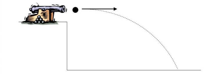
We’ll start with a simple example from phyiscs: the motion of an object under gravity.

Fig. 1 A projectile fired horizontally from a cannon.¶

A projectile fired horizontally at a speed \(v_0 = 5~\mathrm{m/s}\) from an initial height \(y_0 = 200~\mathrm{m}\) follows a trajectory given by the following equations:

\[\begin{split}x(t) = v_0t\\ y(t) = y_0-\frac{1}{2}gt^2\end{split}\]

We will write a program which simulates the trajectory of the projectile. That is, we would like to calulate the \(x\), \(y\) position of the projectile at a given time \(t\).

Let’s start by calculating and printing the \(x\) position at \(t=3~\mathrm{s}\):

# set values of constants

v_0 = 5     # initial velocity
y_0 = 200   # initial y position
g = 9.81    # acceleration due to gravity

# calculate y at time t=3

t = 3
y = y_0 - 0.5 * g * t ** 2

print("t (seconds):", t)
print("y (metres):", y)

t (seconds): 3
y (metres): 155.855

First, we set the value of variables v_0, y_0 and g and t, then calculate the value of y using the expression y_0 - 0.5 * g * t ** 2. Notice that we use * for multiplication but ** for exponentiation!

Finally we use the print fnction to display the output.

Copy the above code and add two lines of code to calculate and print the \(x\) position of the projectile.

By changing the value of t and re-running the code we could calculate the position of the projectile at any time we choose.

Estimate the time the projectile reaches the ground by changing t until y is zero (to the nearest metre)

In the previous workshop, you learned how to write a function. We can avoid having to type the same line of code repeatedly by defining functions for \(x(t)\) and \(y(t)\).

Write two functions for \(x(t)\) and \(y(t)\). Here is some code to get you started:
def x_t(t):
    # x = ...
    return x

Variables

A variable is a way of storing a value in a computer program. Think of a variable like a container and the name of the variable as the label on the container which shows us what is inside.

x = 35

To display the value of a variable, use the print function.

print(x)

35

Python’s inbuilt print() function can take any number of arguments, separated by commas, which will be joined together and printed all at once. In the code above, we pass two arguments to print(): a string ("t (seconds):") which is left as-is, and a variable (t), which is converted into its stored value.

Next we’d like to plot the projectile trajectory on a graph, which will require the calculating x and y for a whole sequence of values of t. To do that, we will use an array.

`Numpy` and arrays¶

An array is a sequence of values that can be manipulated as a single variable. You can think of an array like a vector from mathematics. The following code is identical to previous, except t is now an array of values.

import numpy as np

# set values of constants

v_0 = 5     # initial velocity
y_0 = 200   # initial y position
g = 9.81    # acceleration due to gravity

# calculate y for integer values of t from 0 to 9

t = np.arange(0, 10)
y = y_0 - 0.5 * g * t ** 2

print("t (seconds):", t)
print("y (metres):", y)

t (seconds): [0 1 2 3 4 5 6 7 8 9]
y (metres): [ 200.     195.095  180.38   155.855  121.52    77.375   23.42   -40.345
 -113.92  -197.305]

The first line import numpy as np is required because, by default, Python does not have the capability to work with arrays. To do so, we must import the numpy package which as well as arrays, contains a number of useful mathematical functions which we will use shortly.

Imports

import is used to import a package containing functions not available in Python by default. We only need to import the package once, so it is common practice to put the import statements together at the top of the file.

The function np.arange(0, 10) created an array of 10 time values [0 1 2 3 4 5 6 7 8 9]. This resulted in an array y of 10 distance values [ 100. 95.095 80.38 55.855 21.52 -22.625 -76.58 -140.345 -213.92 -297.305].

Add code to calculate an array x representing the \(x\) positions of the projectile.

Arrays

An array is a sequence of values stored as a single variable. Use the code np.arange(a, b) to create an array of numbers from a to b. Note that b is excluded from the array!

t = np.arange(0, 5)
print(t)

[0 1 2 3 4]

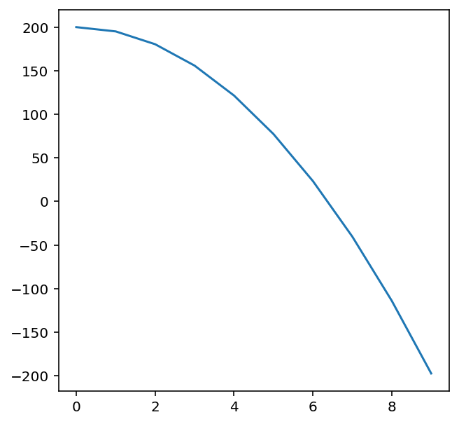
The arrays t and y each contain 10 values. We can plot these values on a line graph:

import matplotlib.pyplot as plt

plt.figure(figsize=(5,5))
plt.plot(t, y)

[<matplotlib.lines.Line2D at 0x7fcba567d340>]

First, we imported another package matplotlib.pyplot which contains useful plotting functions. We then created a 5 by 5 figure and finally plotted t and y on the x- and y-axes respectively.

Plot two more graphs: x against t and y against x. Make sure each is on a separate set of axes!

Plotting

Functions for plotting are contained in a package called matplotlib.pyplot. To create a figure use the function plt.figure and to plot the graph use plt.plot(x, y) where x and y are two arrays of the same length.

Animation¶

Our last step is to generate an animation of the projectile trajectory. The code to achieve this is shown below, but we won’t study it in detail.

from matplotlib import animation
from IPython.display import HTML, display
import random

filename = "animation.gif"
# Number of animation frames equals the length of time array t
frames = len(t)
interval = 100

def ganimate(frame):
    plt.cla()
    plt.scatter(t[frame], y[frame])
    plt.xlim(0, 10)
    plt.ylim(0, 200)
    
fig = plt.figure(figsize=(5, 5))
anim = animation.FuncAnimation(fig, ganimate, frames=frames, interval=interval)
anim.save(filename, writer='imagemagick')
plt.close()

__counter__ = str(random.randint(0,2e9))
display(HTML('<img src="' + filename + '?' + __counter__ + '">'))

The key line is plt.scatter(t[frame], y[frame]) which plots points from the arrays t and y.

The lines plt.xlim(0, 10) and plt.ylim(0, 200) specify the limits of the x- and y-axes respectively.

Copy this code and change it so that it plots the \(x, y\) position of the projectile (you will also need to change the x-axis limits).

Virtual Orrery¶

An orrery is a mechanical device which simulates the motions of heavenly bodies in the Solar System. Your goal is to construct a virtual orrery using Python, a little like the one here. This task is open-ended, and you are unlikely to complete the whole Solar System; just see how far you can get!

Assuming (incorrectly!) that planets follow circular orbits, we can use the following equations to simulation their motion:

\[\begin{split} x(t) = d\cos(2\pi t/p) \\ y(t) = d\sin(2\pi t/p)\end{split}\]

where \(t\) is time in (Earth) days, \(d\) is orbital diameter and \(p\) is the orbital period in (Earth) days. Values of these parameters can be found in the following link:

http://www.astronomynotes.com/tables/tablesb.htm

First, simulate the orbit of the Earth around the sun for. Use np.arange to generate an array of 365 days, then calculate x and y arrays using the equations above. You will need to use the numpy functions np.cos, np.sin and constant np.pi. For d and p use the values in the link above. Plot the orbit on a graph, and animate it.

Next, you could add in the orbits of Mercury and Venus. You will need to introduce new variables for the x and y position of these planets, you could call them x_mercury, y_mercury and so on.

Simulating the moon’s orbit is interesting: the orbit of the moon is relative to Earth, so you will have to add its arrays to the Earth’s arrays.

Take it further….¶

Why not build an orrery out of lego?

Natural Sciences Computing Workshops