Workshop 4 Answers
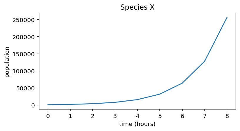
Species X simulation
import numpy as np
import matplotlib.pyplot as plt

r_X = 1
n_hours = 8
initial_population = 1000
pop_X = np.zeros(n_hours + 1)

pop_X[0] = initial_population
for i in range(n_hours):
    pop_X[i + 1] = pop_X[i] + pop_X[i] * r_X

print("Population of species X:", pop_X)
Population of species X: [ 1000. 2000. 4000. 8000. 16000. 32000. 64000. 128000. 256000.]
plt.figure(figsize=(6,3))
plt.plot(pop_X)

plt.xlabel("time (hours)")
plt.ylabel("population")
plt.title("Species X")
Text(0.5, 1.0, 'Species X')
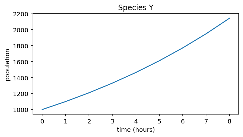
Species Y simulation
# Population with slower growth rate
r_Y = 0.1
n_hours = 8
initial_population = 1000
pop_Y = np.zeros(n_hours + 1)

pop_Y[0] = initial_population
for i in range(n_hours):
    pop_Y[i + 1] = pop_Y[i] + pop_Y[i] * r_Y

print("Population of species Y:", pop_Y)

plt.figure(figsize=(6,3))
plt.plot(pop_Y)

plt.xlabel("time (hours)")
plt.ylabel("population")
plt.title("Species Y")
Population of species Y: [1000.      1100.      1210.      1331.      1464.1     1610.51
 1771.561   1948.7171  2143.58881]
Text(0.5, 1.0, 'Species Y')
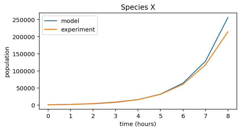
Species X experimental data
# Experimental data collected for X
data_X = np.array([  1.  ,   2.18,   4.45,   8.91,  16.1 ,  31.49,  60.89, 117.58, 214.4 ]) * 1000

# Plot both data and model prediction
plt.figure(figsize=(6,3))
plt.plot(pop_X, label="model")
plt.plot(data_X, label="experiment")

# Figure labels etc
plt.xlabel("time (hours)")
plt.ylabel("population")
plt.title("Species X")
plt.legend()
<matplotlib.legend.Legend at 0x7fae5e96ddf0>
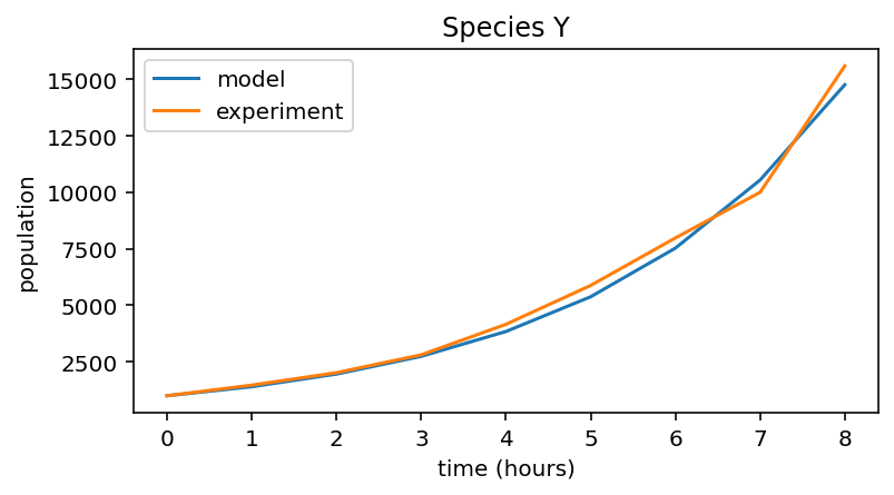
Species Y experimental data
# Predictive model for Y
r_Y = 0.4
n_hours = 8
initial_population = 1000
pop_Y = np.zeros(n_hours + 1)
pop_Y[0] = initial_population
for i in range(n_hours):
    pop_Y[i + 1] = pop_Y[i] + pop_Y[i] * r_Y

# Experimental data collected for Y
data_Y = np.array([  1., 1.47, 2.02, 2.81, 4.16, 5.88, 7.98, 10.00, 15.59 ]) * 1000

# Plot both data and model prediction
plt.figure(figsize=(6,3))
plt.plot(pop_Y, label="model")
plt.plot(data_Y, label="experiment")

# Figure labels etc.
plt.xlabel("time (hours)")
plt.ylabel("population")
plt.title("Species Y")
plt.legend()
<matplotlib.legend.Legend at 0x7fae5e8c8eb0>
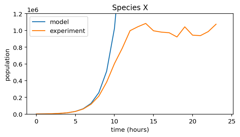
24h experiment
Loading experimental data:
data_X = np.loadtxt("data_exp_X.txt")
print(data_X)
[1.00000000e+03 2.17777342e+03 4.44576258e+03 8.91456547e+03
 1.60958432e+04 3.14897238e+04 6.08883077e+04 1.17580768e+05
 2.14397399e+05 3.81989811e+05 6.03315856e+05 7.87285829e+05
 9.96982461e+05 1.04405640e+06 1.08337178e+06 9.95533440e+05
 9.79746583e+05 9.72332987e+05 9.21969859e+05 1.04273060e+06
 9.43221236e+05 9.37714865e+05 9.85877957e+05 1.07409317e+06]
r_X = 1
n_hours = 24
initial_population = 1000
pop_X = np.zeros(n_hours + 1)

pop_X[0] = initial_population
for i in range(n_hours):
    pop_X[i + 1] = pop_X[i] + pop_X[i] * r_X

plt.figure(figsize=(6,3))
plt.plot(pop_X, label="model")
plt.plot(data_X, label="experiment")

# Uncomment the line below to get a more informative figure
plt.ylim(0, 1.2e6)

plt.xlabel("time (hours)")
plt.ylabel("population")
plt.title("Species X")
plt.legend()
<matplotlib.legend.Legend at 0x7fae5e69aee0>
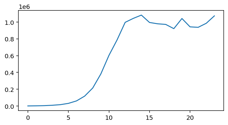
plt.figure(figsize=(6,3))
plt.plot(data_X)
[<matplotlib.lines.Line2D at 0x7fae5e6108b0>]
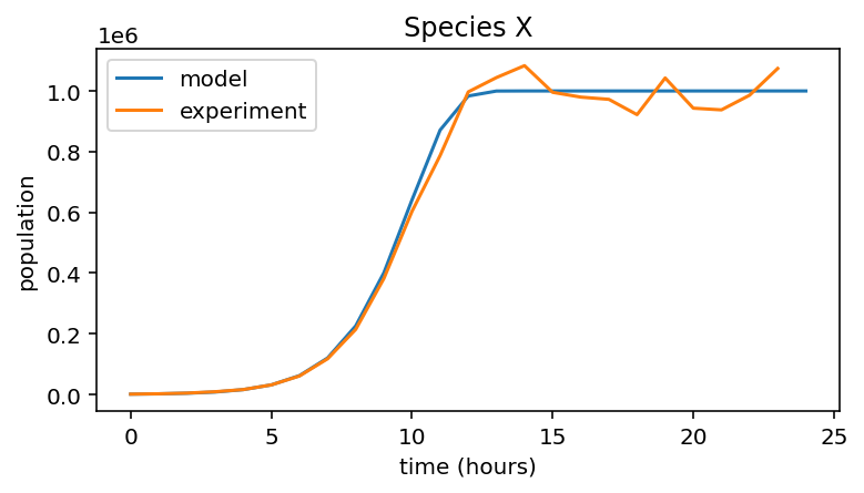
Logistic Growth
Species X
# Set up model for species X
r_X = 1
K_X = 1e6
n_hours = 24
initial_population = 1000

pop_X = np.zeros(n_hours + 1)
pop_X[0] = initial_population

# Simulate logistic growth
for i in range(n_hours):
    pop_X[i + 1] = pop_X[i] + pop_X[i] * r_X * (1 - pop_X[i]/K_X)

# Plot of model and experimental data
plt.figure(figsize=(6,3))
plt.plot(pop_X, label="model")
plt.plot(data_X, label="experiment")

plt.xlabel("time (hours)")
plt.ylabel("population")
plt.title("Species X")
plt.legend()
<matplotlib.legend.Legend at 0x7fae5e5c6dc0>
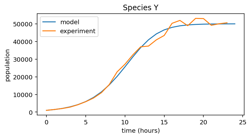
Species Y
# Load 24h experimental data
data_Y = np.loadtxt("data_exp_Y.txt")

# Set up logistic model for species Y
r_Y = 0.45
K_Y = 5e4
n_hours = 24
initial_population = 1000
pop_Y = np.zeros(n_hours + 1)

pop_Y[0] = initial_population
for i in range(n_hours):
    pop_Y[i + 1] = pop_Y[i] + pop_Y[i] * r_Y * (1 - pop_Y[i]/K_Y)

plt.figure(figsize=(6,3))
plt.plot(pop_Y, label="model")
plt.plot(data_Y, label="experiment")

plt.xlabel("time (hours)")
plt.ylabel("population")
plt.title("Species Y")
plt.legend()
<matplotlib.legend.Legend at 0x7fae5e4e3c70>
Exercise
Load experimental data for species A, B, C
data_A = np.loadtxt("data_exp_A.txt")
data_B = np.loadtxt("data_exp_B.txt")
data_C = np.loadtxt("data_exp_C.txt")
# Write a function for logistic growth
def logistic_growth(r, K, x_0, t_max):
    pop = np.zeros(t_max + 1)
    pop[0] = x_0
    for i in range(t_max):
        pop[i + 1] = pop[i] + pop[i] * r * (1 - pop[i]/K)
    return pop

# Growth parameters for each species (adjust values to achieve good fit!)
r = [.9, .4, .7]
K = [5.5e5, 5.5e4, 1e5]
x_0 = [1000, 10000, 1000]
names = ['A', 'B', 'C']

for i, species in enumerate((data_A, data_B, data_C)):

    # Model population growth with species' parameters
    pop = logistic_growth(r[i], K[i], x_0[i], 24)

    # Plot model and data
    plt.figure(figsize=(6,3))
    plt.plot(pop, label="model")
    plt.plot(species, label="experiment")

    plt.xlabel("time (hours)")
    plt.ylabel("population")
    plt.title("Species {0}".format(names[i]))
    plt.legend()
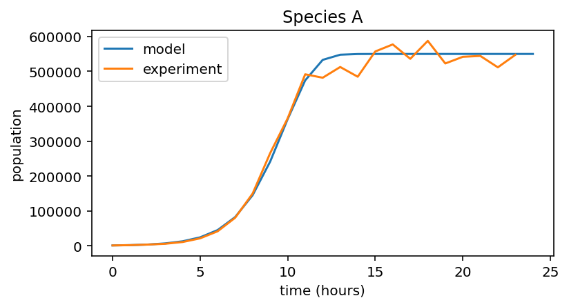
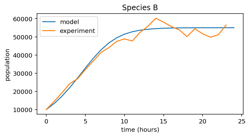
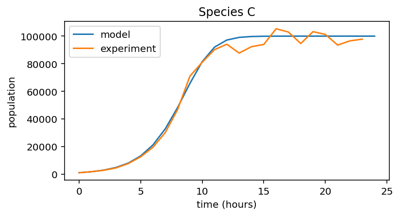
Solution
Species |
Dataset |
r |
K |
\(x_0\) |
|---|---|---|---|---|
1 |
B |
0.4 |
5.5e4 |
10000 |
2 |
C |
0.7 |
1e5 |
1000 |
3 |
A |
0.9 |
5.5e5 |
1000 |
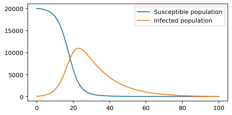
Epidemic model
# Define epidemic model function
def epidemic(a, b, t_max, S_0, I_0):

    S = np.zeros(t_max + 1)
    I = np.zeros(t_max + 1)

    S[0] = S_0
    I[0] = I_0

    for i in range(t_max):
        S[i+1] = S[i] - b * S[i] * I[i]
        I[i+1] = I[i] + b * S[i] * I[i] - a * I[i]

    return S, I
# Create model, vary values of a and b
a = 0.07
b = 0.00002
S_0 = 20000
I_0 = 100

t_max = 100

S, I = epidemic(a, b, t_max, S_0, I_0)

plt.figure(figsize=(6,3))
plt.plot(S, label="Susceptible population")
plt.plot(I, label="Infected population")
# Display legend
plt.legend()
<matplotlib.legend.Legend at 0x7fae5e2dce80>