Arrays
We are already familiar with Python lists, which are used for storing sequences of data. In this lesson we will discover a second data type for storing sequences of data: the Numpy array. Numpy is a Python package designed for working with numerical data. To use it, first import the numpy package and give it the alias np:
import numpy as np
The simplest way to create a numpy array is from a Python list. First create a list of integers or floats, then use the function np.array create an array:
data = [5, 7, 4, 5] # create a Python list
x = np.array(data) # create a numpy array called x containing the same values as 'data'

print(x)
[5 7 4 5]
In many ways numpy arrays are the same as Python lists. We can access individual items by index using square brackets x[i] and sub-arrays using the slice notation x[a:b]. Remember that we include the start index a but exclude the end index b.
y = x[1:3] # extract elements from index 1 to 3
print(y)
[7 4]
Note that numpy arrays can only contain numerical data. Do not try to store a string in an array.
Vector Operations
Arrays support vector operations. These allow us to perform operations on every item in the array simultaneously, without having to use a loop. For example, to add 10 to every element in an array:
y = x + 10
print(y)
[15 17 14 15]
Or to calculate the square of every element of the array:
z = x ** 2
print(z)
[25 49 16 25]
Note this is only possible because x is a numpy array. The following will not work:
a = [1, 2, 3]
b = a + 1 # error since a is a list
We can also perform vector operations on two arrays. For example, to multiply two arrays element-wise:
x = np.array([2, 4, 6, 8])
y = np.array([1, 3, 5, 7])
z = x * y # multiply two arrays element-by-element
print("x * y:", z)
x * y: [ 2 12 30 56]
Numpy Functions
Numpy also includes a number of useful mathematical functions such as np.sin, np.cos and np.exp. In the same way as arithmetic operators, they can be applied to arrays elementwise.
The mathematical constant \(\pi = 3.14\ldots\) is available in numpy as np.pi.
theta = np.array([np.pi/4, np.pi/2]) # create an array with two elements
x = np.sin(theta) # calculate the sin of the array elements
print("theta:", theta)
print("sin(theta):", x)
theta: [0.78539816 1.57079633]
sin(theta): [0.70710678 1.        ]
Creating Numpy Arrays
Unlike Python lists, once a numpy array is created, it cannot be resized. We learnt how to create an empty list [] and add elements one at a time, but this method doesn’t work for arrays. Instead, we must decide the size of the array upfront and create an array of the intended size. Use np.zeros(n) to create an array of n zeros:
z = np.zeros(6) # Create an array of 6 zeros
print(z)
[0. 0. 0. 0. 0. 0.]
Use np.arange(a, b, step) to create an array of evenly spaced numbers ranging from a to b with step size step:
z = np.arange(0, 1, 0.1)
print(z)
[0. 0.1 0.2 0.3 0.4 0.5 0.6 0.7 0.8 0.9]
Use np.linspace(a, b, num) To generate an num evenly spaced numbers between a and b:
z = np.linspace(0, 1, 4)
print(z)
[0. 0.33333333 0.66666667 1. ]
Python lists VS Numpy arrays
Python list |
Numpy array |
|---|---|
Variable size (use |
Fixed size (no |
One-dimensional |
One-dimensional or multidimensional |
Can store multiple data types (strings, floats, ints, other lists) |
Can store only numerical data of a single type |
Does not support vector operations |
Supports vector operations |
Slow |
Fast |
Example: Damped Oscillator
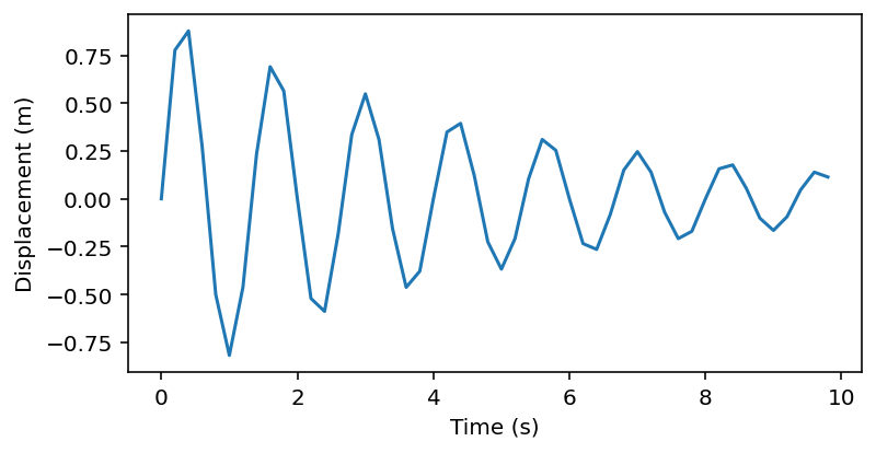
The following equation describes the motion of a damped linear oscillator, where \(t\) is time and \(x\) is displacement.
We will plot the trajectory of the oscillator, given \(\alpha=0.2\) and \(f=1.5\).
alpha = 0.2
f = 1.5
time = np.arange(0, 10, 0.2) # create an array of evenly spaced time points between 0 and 10
x = np.exp(-alpha * time) * np.sin(np.pi * f * time) # calculate the displacement x using vector operations

import matplotlib.pyplot as plt
plt.figure(figsize=(6,3))
plt.plot(time, x)
plt.xlabel("Time (s)")
plt.ylabel("Displacement (m)")
Text(0, 0.5, 'Displacement (m)')

Multi-Dimensional Arrays
We specifiy 2 dimensional arrays using a list whose elements are the rows of the array. For example, to specify the following 2-d array:
data = [[1, 2, 3], [4, 5, 6]]
x = np.array(data)

print(x)
[[1 2 3]
 [4 5 6]]
data is a nested list. Each element of data is itself a list representing a row of the array. Note that we can make this a lot clearer by writing each row on a separate line:
x = np.array([[1, 2, 3],
              [4, 5, 6]])
print(x)
[[1 2 3]
 [4 5 6]]
Individual array elements are accessed using the [] index notation, passing one index per dimension. x[i,j] returns the element in row i, column j:
z = x[0,1]
print(z)
2
Array slicing
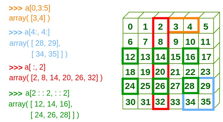
Use a colon : in place of the index to extract an entire row or column from an array. This is called taking a ‘slice’ from the array.
first_row = x[0,:]
print(first_row)
[1 2 3]
first_column = x[:,0]
print(first_column)
[1 4]
Supply starting and ending indexes to extract parts of an array. Remember that in Python, we always include the start index but exclude the end index.
first_two_columns = x[:,:2]
print(first_two_columns)
[[1 2]
 [4 5]]
See the figure below for an illustration of slicing a 2-d array.

Fig. 2 Numpy array slicing
Example: Population Growth
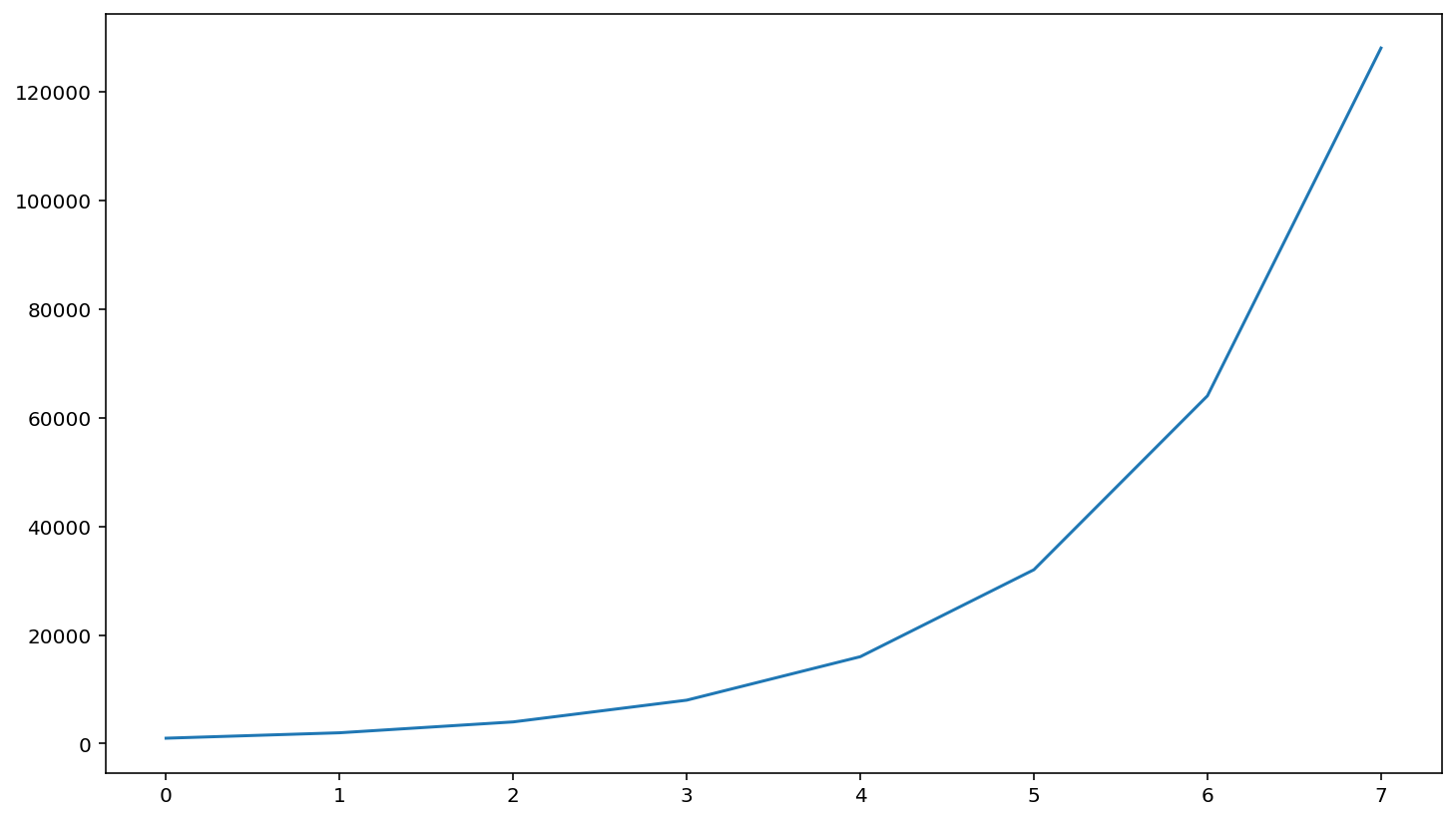
The following equation describes the rate of growth of a population \(x_i\) of hourly growth \(r\).
Previously we simulated population growth using Python lists. Below is how we might do exactly the same using arrays.
import numpy as np
import matplotlib.pyplot as plt

# set parameter values
r = 1
n_hours = 8
initial_population = 1000

# create array of time points
t = np.arange(0, n_hours, 1)

pop = np.zeros(n_hours)
pop[0] = initial_population

# run simulation
for i in range(n_hours - 1):
    pop[i+1] = pop[i] + pop[i] * r

plt.plot(t, pop)
[<matplotlib.lines.Line2D at 0x7f429bf560d0>]

