Image Processing
This tutorial will examine how to use Python and Numpy to process images, which can be expressed as 2 or 3 dimensional arrays.
More Array Functions
First we look at another method of constructing 2d arrays, by constructing one row at a time. Suppose we want to create the following array, where the first row is powers of 2, the second row is powers of 3, and so on:
We create a zero array of the desired dimensions using the function np.zeros:
import numpy as np

a = np.zeros((3, 4))
print(a)
[[0. 0. 0. 0.]
 [0. 0. 0. 0.]
 [0. 0. 0. 0.]]
Notice the double brackets, which are necessary because the function np.zeros takes a tuple as a parameter.
Next, we create each of the individual rows as 1 x 4 arrays:
x = np.arange(0, 4)
row1 = 2 ** x
print(row1)
row2 = 3 ** x
print(row2)
row3 = 4 ** x
print(row3)
[1 2 4 8]
[ 1  3  9 27]
[ 1  4 16 64]
Finally, we assign each row to the correct row in a using slice notation:
a[0, :] = row1
a[1,:] = row2
a[2,:] = row3

print(a)
[[ 1.  2.  4.  8.]
 [ 1.  3.  9. 27.]
 [ 1.  4. 16. 64.]]
shape Method
Given an array, we can determine its dimensions using the shape method, which returns a tuple:
s = a.shape
print(s)

x = s[0]
y = s[1]

print("first dimension:", x)
print("second dimension:", y)
(3, 4)
first dimension: 3
second dimension: 4
Axis Methods
The method np.sum allows us to calculate the sum of the elements in an array. If your array is 2-dimensional, it is often useful to calculate the sum in one dimension only, to return a 1-dimensional array. This can be achieved using the axis parameter of the sum function:
sum_of_rows = np.sum(a, axis=0)
print(sum_of_rows)
[ 3. 9. 29. 99.]
This method has performed the vector sum of the rows of a, [1, 2, 4, 8] + [1, 3, 9, 27] + [1, 4, 16, 64]. Element i of the result is the sum down the column i of a. The parameter axis=0 determines that it is the 1st (counting from 0) dimension that should be aggregated.
To perform the aggregation along the second dimension, use axis=1.
sum_of_columns = np.sum(a, axis=1)
print(sum_of_columns)
[15. 40. 85.]
Other methods that take the axis parameter include np.max and np.mean.
Images
An image file is essentially a 3-dimensional array where each element represents colour intensity of each pixel. The first two dimensions correspond to the x and y co-ordinates of each pixel, and the third dimension corresponds to its RGBA value (R=red, G=Green, B=Blue and A=alpha which encodes transparency).
The file bw.png is an 8 by 8 pixel image (download):
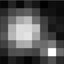
First we import the module matplotlib.image and use the imread function to convert it to an array.
import matplotlib.image as mpimg # import the image module

x = mpimg.imread("bw.png") # read the image into an array

print("shape:", x.shape)
shape: (8, 8, 4)
This is a three dimensional array where x[i,j,0] is the R value, x[i,j,1] is the G value, x[i,j,2] is the B value and x[i,j,3] is the alpha (transparency) value. x[0, 0, :] extracts all four values for the (0, 0) pixel as a 1 x 4 array:
print(x[0, 0, :])
[0.02352941 0.02352941 0.02352941 1. ]
This is a greyscale image, so all the colour values are identical and the alpha value is 1 (100% opaque). We can aggregate along the third (number 2) axis to sum the colour values and return a 2-dimensional array. (The round function is used to make the printed array easier to read by reducing the number of decimal places displayed).
z = np.sum(x, axis=2)
print(np.round(z, 1))
[[1.1 1.4 1.1 1.5 1.3 1.  1.2 1.1]
 [1.5 1.8 2.  2.1 1.8 1.2 1.2 1.1]
 [1.8 2.4 3.  3.2 2.3 1.7 1.4 1.2]
 [1.9 3.1 3.6 3.6 3.3 1.8 1.3 1.3]
 [2.  3.2 3.6 3.7 3.  2.  1.7 1.2]
 [1.8 2.3 3.  3.1 2.4 2.3 2.5 1.7]
 [1.4 1.9 2.  1.9 1.8 2.4 4.  2.3]
 [1.1 1.4 1.2 1.1 1.2 1.6 1.9 1.5]]
Particle Tracking
Many scientific experiments require the capture of mages, for example microscopic images of biological tissue slices, or photographs of astronomical objects images. Computers enable us to automate many of the processes associated with analysing such images, such as the automatic segmentation and labelling of cells in a tissue slice or identification of astronomical objects.
We will be using Python image processing techniques to reproduce part of a famous experiment: Perrin’s experiment to measure Avogadro’s Number. In this experiment, images of tiny particles are recorded through a microscope.
This lesson is based in part on an assignment from Princeton University and you are encouraged to read it for reference.
Read in an image file and convert it to a
numpyarray.Convert the array to greyscale by averaging along the last dimension
Classify the pixels as foreground or background
Find the particle locations
Repeat for all images and plot a graph of particle location against time
Read the Image File
import numpy as np
import matplotlib.pyplot as plt
import matplotlib.image as mpimg # import the image module

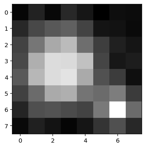
x = mpimg.imread("bw.png") # read the image into an array
plt.figure(figsize=(4,4))
plt.imshow(x)
<matplotlib.image.AxesImage at 0x7fe3c5958820>
Reduce to greyscale
print("Dimensions:", x.shape)
Dimensions: (8, 8, 4)
We will reduce the array to 2-dimensions by summing the last dimension:
z = np.sum(x, 2) # sum the RGBA values for each pixel
print(np.round(z, 1))
[[1.1 1.4 1.1 1.5 1.3 1.  1.2 1.1]
 [1.5 1.8 2.  2.1 1.8 1.2 1.2 1.1]
 [1.8 2.4 3.  3.2 2.3 1.7 1.4 1.2]
 [1.9 3.1 3.6 3.6 3.3 1.8 1.3 1.3]
 [2.  3.2 3.6 3.7 3.  2.  1.7 1.2]
 [1.8 2.3 3.  3.1 2.4 2.3 2.5 1.7]
 [1.4 1.9 2.  1.9 1.8 2.4 4.  2.3]
 [1.1 1.4 1.2 1.1 1.2 1.6 1.9 1.5]]
Tresholding
The next step is to classify each pixel as ‘foreground’ (belonging to a particle) or ‘background’. We do this by setting each pixel to 1 if it is above a threshold value, and 0 otherwise. But what threshold value should we choose? It certainly must lie between the minimum and maximum values of the array.
print("Min:", np.min(z))
print("Max:", np.max(z))
Min: 1.0
Max: 4.0
The threshold must lie between 1 and 4. Let’s try a value of 2.
thres = 2
x_thres = z > thres # Determine pixels which are above the threshold
print(x_thres)
plt.figure(figsize=(4,4))
plt.imshow(x_thres) # Note that in Python True = 1 and False = 0
[[False False False False False False False False]
 [False False  True  True False False False False]
 [False  True  True  True  True False False False]
 [False  True  True  True  True False False False]
 [ True  True  True  True  True False False False]
 [False  True  True  True  True  True  True False]
 [False False False False False  True  True  True]
 [False False False False False False False False]]
<matplotlib.image.AxesImage at 0x7fe3c58e8040>
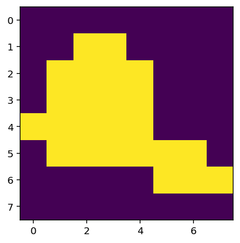
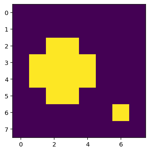
We would like to identify the largest blob (the top left one). We will increase the value of thres so that there are two distinct blobs in the thresholded image.
thres = 2.5
x_thres = z > thres # Determine pixels which are above the threshold
print(x_thres)
plt.figure(figsize=(4,4))
plt.imshow(x_thres) # Note that in Python True = 1 and False = 0
[[False False False False False False False False]
 [False False False False False False False False]
 [False False  True  True False False False False]
 [False  True  True  True  True False False False]
 [False  True  True  True  True False False False]
 [False False  True  True False False False False]
 [False False False False False False  True False]
 [False False False False False False False False]]
<matplotlib.image.AxesImage at 0x7fe3c58cb760>
Blob Location
The next step is the determine the location of the largest identified blob. Fortunately there are functions available in the scipy.ndimage package which do just that. First, use the function label to generate an array in which each element is a number identifying which connected blob the pixel belongs to. In this case, there are two blobs, so every pixel is labelled 1 or 2 if it belongs to one of the blobs, or 0 if it belongs to neither.
import scipy.ndimage as sn # import the scipy.ndimage package
x_labels, n = sn.label(x_thres) # generate
print("number of blobs:", n)
print(x_labels)
number of blobs: 2
[[0 0 0 0 0 0 0 0]
 [0 0 0 0 0 0 0 0]
 [0 0 1 1 0 0 0 0]
 [0 1 1 1 1 0 0 0]
 [0 1 1 1 1 0 0 0]
 [0 0 1 1 0 0 0 0]
 [0 0 0 0 0 0 2 0]
 [0 0 0 0 0 0 0 0]]
Next, use the sn.sum function to generate an array containing the size (in number of pixels) of each blob.
sizes = sn.sum(x_thres, x_labels, range(1, n+1))
print("sizes:", sizes)
sizes: [12. 1.]
So blob 1 has 9 pixels and blob 2 has 1 pixel.
np.argmax returns the index of the largest blob:
idx = np.argmax(sizes) # get the index of the largest blob
print("index:", idx)
index: 0
Note that the indexes of the sizes array are counted from 0 to n-1, whereas the labels are counted from 1 to n, so index idx corresponds to the blob with label idx + 1.
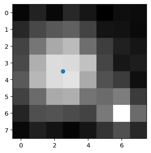
Next we determine the location of the largest blob using the sn.center_of_mass function, which returns the co-ordinates of the centre of a blob.
location = sn.center_of_mass(x_thres, x_labels, idx + 1) # determine the coordinates of the largest blob
print("location:", location)
location: (3.5, 2.5)
Note
The location variable is a tuple. A tuple is the same as a list, and we use the same square bracket notation to access elements, such as location[0]. But:
When defining a tuple we use round brackets
()instead of square brackets[].location = (1, 4).A tuple is immutable, meaning its elements cannot be changed.
location[0] = 5results in an error.
Finally we will mark the location of the centre of the largest blob using plt.scatter. Arrays indices are ordered row then column which is opposite to x-y ordering for the scatter plot, so we have to reverse the ordering of the location elements when plotting.
plt.figure(figsize=(4,4))
plt.imshow(x)
# arrays are indexed [column, row] whereas scatter plots are ordered [x, y]
# so we need to reverse the order of the indices
plt.scatter(location[1], location[0])
<matplotlib.collections.PathCollection at 0x7fe3b4ef6e50>
In this week’s exercises you will repeat this procedure using a sequence of real experimental images of particles exhibiting Brownian motion.
