.md .pdf

Contents

6. Integration

6.1. Introducing Integration

6.1.1. The “anti-derivative”

Consider the function \(\cos(x)\). We know that this function can be obtained by differentiating \(\sin(x)\). Therefore, we could think of \(\sin(x)\) as the “anti-derivative” of \(\cos(x)\). After differentiating \(\sin(x)\), the “anti-derivative” takes us back to where we started.

Well… nearly. We could also obtain \(\cos(x)\) by differentiating \(\sin(x)+2\), so we cannot say that \(\sin(x)\) is the unique anti-derivative of \(f(x)\).

In general, for a given function \(f(x)\),

if \(\frac{\mathrm{d}F}{\mathrm{d}x} = f(x)\), then \(F(x)+c\) is an antiderivative of \(x\),

where \(c\) is an arbitrary constant.

Being able to “spot” anti-derivatives is a tremendously useful (and often under-utilised) trick.

Practice

Note: these are not “integration questions”. You only need to use your knowledge of differentiation, and the concept of the anti-derivative, as described above.

1. \(\sec^2(x)\)

2. \(x^3\)

3. \(\sin(3x)\)

4. \(e^{a x}\)

5. \(x \sqrt{x^2-1}\)

6. \(\frac{x}{x^2+1}\)

7. \(\frac{\sin(x)}{\cos(x)}\)

8. \(\cosh(x)\sinh^2(x)\)

6.1.2. Area under the curve

Fig. 6.1 shows how the area under a curve \(f(x)\) between \(x=a,b\) may be estimated by drawing rectangles of equal width \(\Delta x\). Formally, we may write that:

(6.1)\[\textrm{Area} = \sum_{j=0}^{n-1}f(x_n)\Delta x \textrm{, where }x_0=a, x_n=b, \Delta x = \frac{b-a}{n}\]

The expression simply states that we add up the rectangles with width \(\Delta x\) and height \(f(x_n)\). As \(\Delta x\rightarrow 0\) the area approximation becomes more accurate.

We call \( \lim_{\Delta x \rightarrow 0}\sum_{j=0}^{n-1}f(x_j)\Delta x\) the integral of \(f\) with respect to \(x\) and we denote it by:

(6.2)\[ \displaystyle \int_a^b f(x)\mathrm{d}x\]

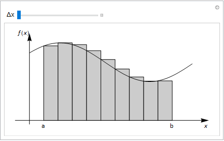
Fig. 6.1 Rectangles drawn under the curve \(f(x)\) can be used to approximate the area. The thinner the rectangles, the better the approximation. Integration is the equivalent to this approach as the width of the rectangles, \(\Delta x \rightarrow 0\).

It can be proved that integration and anti-differentiation are essentially the same thing. This result is known as the “fundamental theorem of calculus”. In fact, the theorem comes in two parts. The first part, given in the box below, allows the definite integral to be determined by evaluating an anti-derivative at integration limits. The second part (not given here) essentially proves that every continuous function has an anti-derivative, which can be found by integration. For some functions, such as \(e^{-x^2}\), we might not be able to express the integral in terms of elementary functions, but we know it exists (and we can use successive approximation techniques either analytically or numerically to estimate them).

Definition

The First Fundamental Theorem of Calculus (FTC1)

If \(F\) is an anti-derivative of \(f\), then \(\displaystyle \int_a^b f(x) \textrm{d}x = F(b) - F(a)\) gives the area between the curve \(f(x)\) and the x-axis between \(x=a\) and \(x=b\).

Symbol	Meaning	Notes
\(\textrm{d}x\)	“with respect to x” The integration is along the x-axis. We say that x is the “integration variable”	Do not forget to write this, or the integral has no meaning.
\(\displaystyle \int\)	Integration operator	An operator acs on a function in some way. For example, \(\frac{\textrm{d}}{\textrm{d}x}\) is also an operator.
\(f(x)\)	Integrand	The function to be integrated.
\(a, b\)	The limits of integration.	If the integral has limits then it is called a definite integral and has a single value for the solution. If the integration does not have limits then it is called an indefinite integral, and you can only compute the result to within an arbitrary constant.

6.1.3. Signed and unsigned areas

Note that the heights of the rectangles in Fig. 6.1 are given by \(f(x)\), and so if \(f(x)<0\) then the result will be negative. In many examples, positive and negative areas cancel. For instance,

(6.3)\[\displaystyle \int_0^{2\pi}\sin(x)\mathrm{d}x = 0 \textrm{, since } \displaystyle \int_0^{\pi}\sin(x)\mathrm{d}x = 2 \textrm{ and } \displaystyle \int_{\pi}^{2\pi}\sin(x)\mathrm{d}x = -2\]

If you want the total (unsigned) area between the curve and the axis, then you can work with the modulus of the function,

(6.4)\[\displaystyle \int_a^b |f(x)|\mathrm{d}x\]

The easiest way to do this is to split up the region of integration into areas where \(f(x)>0\) and areas where \(f(x)<0\). For example,

(6.5)\[\displaystyle \int_0^{2\pi}|\sin(x)|\mathrm{d}x = \displaystyle \int_0^{\pi}\sin(x)\mathrm{d}x+ \displaystyle \int_{\pi}^{2\pi}-\sin(x)\mathrm{d}x = 2+2 =4\]

The results are illustrated in Fig. 6.2 below.

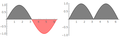
Fig. 6.2 The plot on the left shows \(\sin(x)\) for \(x\in[0,2\pi]\). The black and red signed areas (2,-2) cancel when the integral is performed. The plot on the right shows \(|\sin(x)|\) for \(x\in[0,2\pi]\). The black signed are both positive and so the integral is 2+2=4.

Similarly, if we perform the integration along the x-axis in the negative direction, then the quantities \(\Delta x\) are negative, and so we end up with a negative signed area when \(f(x) > 0\).

FTC1 also confirms that \(\displaystyle \int_b^a f(x) \textrm{d}x = -\displaystyle \int_a^b f(x) \textrm{d}x\).

6.1.4. Area between two curves

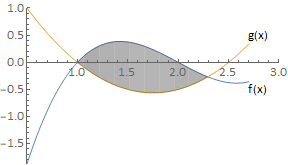
Fig. 6.3 Where \(f(x) >= g(x)\) the integral \(\displaystyle \int (f(x)-g(x)) \textrm{d}x\) gives the area between the two curves.

Practice

1. a) Find the tangent to the curve \(y=25-x^2\) at the point where \(x=2\).

b) Calculate the value of \(x\) where the tangent meets the x-axis.

c) Find the area of the region bounded by the tangent, the curve and the x-axis.

2. Calculate the area of the region bounded by the curves \(x = -y^2 + 10\) and \(x = (y-2)^2\).

6.1.5. Solutions to this chapter

6.1.5.1. Anti-derivative questions

1. We should recognise that \(\sec^2(x)\) is obtained by differentiating \(\tan(x)\) and so the anti-derivative is \(F(x)=\tan(x)+c\).

2. If we differentiate \(x^4\) we obtain \(4x^3\) which is nearly what we want, but not quite. Trying \(\frac{\mathrm{d}}{\mathrm{d}x} \left(\frac{1}{4} x^4\right)\) instead gets the result \(x^3\) and so the anti-derivative of \(x^3\) is \(\frac{1}{4} x^4+c\).

3. By the chain rule, \(\frac{\mathrm{d}}{\mathrm{d}x} \cos(3x)=-3\sin(3x)\), and so the anti-derivative is \(-\frac{1}{3}\cos(3x)+c\).

4. \(\frac{\mathrm{d}}{\mathrm{d}x}e^{a x}=a e^{a x}\) and so the anti-derivative is \(\frac{1}{a} e^{a x}+c\).

5. Now we rely on our expertise with the chain rule. The chain rule tells us that \(f(g(x))^{\prime}=g^{\prime}(x)f^{\prime}(g)\) and so the anti-derivative of \(g^{\prime}(x)f^{\prime}(g)\) is \(f(g(x))+c\). In particular, if we differentiate \(g^{3/2}\) where \(g=x^2-1\), we obtain \((2 x) \frac{3}{2} g^{1/2}\) and so the anti-derivative of \(x g^{1/2}\) is \(\frac{1}{3} g^{3/2}+c =\frac{1}{3} (x^2-1)^{3/2}+c\). (CHECK IT: you need to be awesome at differentiation to be good at integration).

6. By the same rationale as question 5, we try \(\frac{\mathrm{d}}{\mathrm{d}x} \ln(x^2+1)=\frac{2x}{x^2+1}\) and so the anti-derivative is \(\frac{1}{2} \ln(x^2+1)+c\).

7. The anti-derivative is \(-\ln(cos(x))+c\). In general, the anti-derivative of an expression of the form \(\frac{f^{\prime}(x)}{f(x)}\) is \(\ln(f(x))+c\).

8. The anti-derivative is \(\frac{1}{3} \sinh^3(x)+c\).

6.1.5.2. Integration Questions

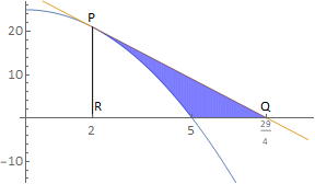
The tangent is \(y=29-4x\), which intersect that x-axis at \(x=29/4\) (see diagram below). The required area is given by PQR - \( \displaystyle \int_2^5(25-x^2)\mathrm{d}x = \frac{1}{2}\left(\frac{21}{4}21 - \left[25x-\frac{x^3}{3}\right]_2^5\right) = \frac{153}{8}\)

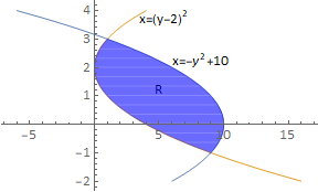
The curves intersect at (1,3) and (9,-1). It is easier to calculate the enclosed area by integrating parallel to the y-axis.

\(R = \displaystyle \int_{y=1}^3\left[(10-y^2)-(y-2)^2\right]\mathrm{d}y = \displaystyle \int_1^3(-2y^2+4y+6)\mathrm{d}y =\frac{64}{3}\)

6.2. Integration Rules

6.2.1. Integration by substitution

Definition

For an indefinite integral:

\(\displaystyle \int f(x) \textrm{d}x = \displaystyle \int f(x) \frac{\mathrm{d}x}{\mathrm{d}u}\mathrm{d}u+c\)

For a definite integral: \(\displaystyle \int_a^b f\mathrm{d}x=\displaystyle \int_{u(a)}^{u(b)}f\frac{\mathrm{d}x}{\mathrm{d}u}\mathrm{d}u\)

Don’t forget to change the limits for definite integration!

The result can be proved using the chain rule and fundamental theorem of calculus.

The idea of using a substitution is that we convert a difficult integral w.r.t \(x\) to an easier one w.r.t \(u\) Note that \(f \frac{\mathrm{d}x}{\mathrm{d}u}=f\biggr/\frac{\mathrm{d}u}{\mathrm{d}x}\) and so the substitution \(u\) can be chosen to eliminate a factor from \(f\).

Examples

1. To calculate \( \displaystyle \int x\sqrt{x^2-1}\mathrm{d}x\) we can try the substitution \(u=x^2-1\). This substitution will eliminate the factor \(x\) and will simplify the expression \(\sqrt{x^2-1}\). We find that

\( \frac{\mathrm{d}u}{\mathrm{d}x}=2x\) and so \(\frac{\mathrm{d}x}{\mathrm{d}u}=\frac{1}{2x}\)

\( x\sqrt{x^2-1}\mathrm{d}x=\displaystyle \int\frac{1}{2}u^{1/2}\mathrm{d}u=\frac{1}{3}u^{3/2}+c=\frac{1}{3}(x^2-1)^{3/2}+c\)

This is the same result we found by inspection in the previous chapter.

2. To calculate the definite integral \( I=\displaystyle \int_1^3\frac{1}{2x+1}\mathrm{d}x\) we will use the substitution \(u=2x+1\). (This problem could also be solved by inspection)

When \(x=1\), \(u=3\). When \(x=3\), \(u=7\).

Hence, the result is \(I=\displaystyle \int_{u=3}^{u=7}\frac{1}{u}\biggr/\frac{\mathrm{d}u}{\mathrm{d}x}\mathrm{d}u =\frac{1}{2}\displaystyle \int_3^7\frac{1}{u}\mathrm{d}u=\frac{1}{2}\biggr[\ln(u)\biggr]_3^7=\frac{1}{2}\ln\biggr(\frac{7}{3}\biggr)\)

3. To calculate an expression of the form \( I=\displaystyle \int (ax+b)(cx+d)^n\mathrm{d}x\) we can make the substitution \(u=cx+d\). This gives \( I=\displaystyle \int\left(a\frac{u-d}{c}+b\right)u^n\frac{1}{c}\mathrm{d}u=\frac{1}{c^2}\displaystyle \int(au+bc-ad)u^n\mathrm{d}u\)

By polynomial expansion \( I=\frac{1}{c^2}\displaystyle \int(a u^{n+1}+(bc-ad)u^n)\mathrm{d}u=\frac{1}{c^2}\left[\frac{a u^{n+2}}{n+2}+\frac{bc-ad}{n+1}u^{n+1}\right]\)

Rewriting in terms of \(x\) finally gives \(I = \frac{(cx+d)^{n+1}}{c^2}\left[\frac{a(cx+d)}{n+2}+\frac{bc-ad}{n+1}\right]\)

6.2.1.1. Integral of \(\frac{1}{x}\)

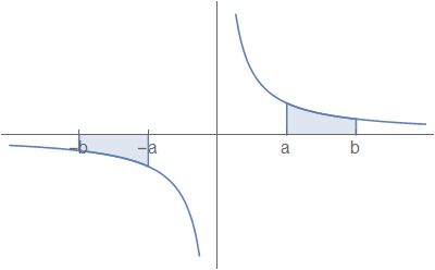
Fig. 6.4 The plot of \(y=\frac{1}{x}\), showing limits of integration ±a and ±b.

\(\displaystyle \int_{-b}^{-a}\frac{1}{x}\mathrm{d}x = -\displaystyle \int_a^b\frac{1}{x}\mathrm{d}x = \displaystyle \int_b^a\frac{1}{x}\mathrm{d}x = \displaystyle \int_{-b}^{-a}\frac{1}{|x|\mathrm{d}x}\)

So, \(\displaystyle \int\frac{1}{x}=\ln(|x|)+\mathrm{const}\), \(\forall x\), provided that the range of integration does not cross the vertical axis.

\(\displaystyle \int_{-a}^a\frac{1}{x}\mathrm{d}x\) is undefined, though we can define the Cauchy principal value of this integral as

\(\lim_{\epsilon\rightarrow 0^{+}}\left(\displaystyle \int_{-a}^{-\epsilon}\frac{1}{x}\mathrm{d}x+\displaystyle \int_{\epsilon}^a\frac{1}{x}\mathrm{d}x\right)=0\)

6.2.2. Integration by parts

Definition

For an indefinite integral:

\(\displaystyle \int u\frac{\mathrm{d}v}{\mathrm{d}x}\mathrm{d}x = uv-\displaystyle \int v\frac{\mathrm{d}u}{\mathrm{d}x}\mathrm{d}x+c\)

For a definite integral:

\(\displaystyle \int_a^b u\frac{\mathrm{d}v}{\mathrm{d}x}\mathrm{d}x=\biggr[uv\biggr]_a^b-\displaystyle \int_a^b v\frac{\mathrm{d}u}{\mathrm{d}x}\mathrm{d}x\)

This result can be proved using the produc rule and the fundamental theorem of calculus.

\(\displaystyle \int \mathrm{d}(uv)=\displaystyle \int u\mathrm{d}v+\displaystyle \int v\mathrm{d}u \rightarrow uv=\displaystyle \int u\mathrm{d}v=\displaystyle \int v\mathrm{d}u\)

For a handy rule of thumb for choosing which term to differentiate when applying this method, do a web search for “LIATE”.

Examples

1. To calculate \(\displaystyle \int x e^{-x}\mathrm{d}x\) we let \(u=x\), \(\frac{\mathrm{d}v}{\mathrm{d}x}=e^{-x}\) in the formula for integration by parts.

Then,

\(\frac{\mathrm{d}u}{\mathrm{d}x}=1\) (which is simpler)

\(v=-e^{-x}\) (which is no more complicated)

So \( \displaystyle \int x e^{-x}\mathrm{d}x=-x e^{-x}+\displaystyle \int e^{-x}\mathrm{d}x = -e^{-x}(x+1)+\mathrm{const}\)

2. To calculate \( \displaystyle \int x^2 e^{-x}\mathrm{d}x\), we let \(u=x^2\), \(\frac{\mathrm{d}v}{\mathrm{d}x}=e^{-x}\)

Then,

\(\frac{\mathrm{d}u}{\mathrm{d}x}=2x\) (which is simpler)

\(v=-e^{-x}\) (which is no more complicated)

So \( \displaystyle \int x^2 e^{-x}\mathrm{d}x=-x^2 e^{-x}+2\displaystyle \int x e^{-x}\mathrm{d}x\)

From the previous example, we know this result is

\( \displaystyle \int x^2 e^{-x}\mathrm{d}x=-e^{-x}(x^2+2x+2)\)

3. To calculate \( I=\displaystyle \int \arcsin(x)\mathrm{d}x\) we play a trick:

Let \(u=\arcsin(x)\), \(\frac{\mathrm{d}v}{\mathrm{d}x}=1\)

Then,

\(x=\sin(u)\), so \(\frac{\mathrm{d}x}{\mathrm{d}u}=\cos(u)=\sqrt{1-x^2}\)

We should be cautious here. The positive square root is chosen because \(\sin(x)\) is increasing throughout its domain

\(v=x\)

This gives

\( I=x\arcsin(x)-\displaystyle \int\frac{x}{\sqrt{1-x^2}}\mathrm{d}x\)

The remaining integral can be calculated by inspection, or with the substitution \(u=1-x^2\).

\(I=x \arcsin(x)+\sqrt{1-x^2}+\mathrm{const}.\)

6.2.3. Integration by partial fractions

Composing fractions means putting everything together. For example

(6.6)\[\frac{2}{x+1}+\frac{3}{x+2}=\frac{2(x+2)+3(x+1)}{(x+1)(x+2)}=\frac{5x+7}{x^2+3x+2}\]

Decomposition is the reverse process, i.e. taking thr fraction apart.

As an introductory example, lets try to decompose \(\frac{11x+3}{x^2 + 3x + 2}\) into partial fractions. by comparing with (6.6) we can anticipate that the decomposition will have the form \(\frac{A}{x+1}+\frac{B}{x+2}\), which can be composed to give:

\[\frac{A}{x+1}+\frac{B}{x+2}=\frac{A(x+2)+B(x+1)}{(x+1)(x+2)}=\frac{(A+B)x+(2A+B)}{x^2+3x+2}\]

To obtain the required fraction, we need \((A+B)x+(2A+B)=11x+3\).

This can be achieved by choosing \(A=-8\), \(B=19\). Hence, the result is

\[\frac{11x+3}{x^2+3x+2}=\frac{-8}{x+1}+\frac{19}{x+2}\]

This technique allows us to easily integrate:

\[\displaystyle \int\frac{11x+3}{x^2+3x+2}\mathrm{d}x=\displaystyle \int\left(\frac{-8}{x+1}+\frac{19}{x+2}\right)\mathrm{d}x=-\ln|x+1|+19\ln|x+2|+c\]

Further Example

Now consider the fraction \(\frac{2}{(x^2-1)(x+2)}\)

It can be decomposed as follows:

\(\frac{2}{(x^2-1)(x+2)}=\frac{Ax+B}{x^2-1}+\frac{C}{x+2}\)

This gives \((Ax+B)(x+2)+C(x^2-1)=2\) and by equating coefficients on the left and right sides we obtain

\(\frac{2}{(x^2-1)(x+2)}=\frac{2(2-x)}{x^2-1}+\frac{2}{x+2}\)

However, we can decompose this fraction further by noting that \((x^2-1)=(x+1)(x-1)\).

The full decomposition is

\(\frac{2}{(x^2-1)(x+2)}=\frac{1}{3(x-1)}-\frac{1}{1+x}+\frac{2}{3(x+2)}\)

(which we could integrate as a sum of logarithmic terms).

Partial Fractions: Tips

1. If the degree of the numerator \(m\) is greater than (or equal to) the degree of the denominator \(n\), split off the leading terms in the form of a polynomial of degree \(m-n\).

2. Split up the remaining fraction so that the degree of each numerator is one less than the degree of the denominator.

3. To find the unknown constants, combine the fractions on the right hand side and equate the coefficients in the numerators on the left and right.

Example

\(\frac{2}{x^2-1}= \frac{A}{x-1} + \frac{B}{x+1}\)

\(\frac{x^2+3x+4}{(x+1)(x+3)}= A + \frac{B}{x+1} + \frac{C}{x+3}\)

\(\frac{3x^3+3}{(x+1)(x+3)} = (Ax +B) +\frac{C}{x+1}+ \frac{D}{x+3}\)

\(\frac{2}{(x^2+1)(x-1)} = \frac{Ax+B}{x^2+1}+\frac{C}{x-1}\)

\(\frac{2x+3}{(x+1)^2} = \frac{A}{(x+1)^2}+\frac{B}{x+1}\)

6.2.4. Reduction formula examples

1.

\[I_n = \displaystyle \int x^n e^x\mathrm{d}x = x^n e^x - n \displaystyle \int x^{n-1}e^x\mathrm{d}x\]

That is, \(I_n = x^n e^x - n I_{n-1}\), and \(I_0 = \displaystyle \int e^x\mathrm{d}x = e^x + k\)

e.g.

\[I_4 = e^x(x^4- 4x^3+4(3)x^2 - 4(3)(2)x +4(3)(2)(1))+\mathrm{const}\]

2.

\[I_n = \displaystyle \int_0^{\pi/2}\cos^{n}(x)\mathrm{d}x = \displaystyle \int_0^{\pi/2}\cos(x)\cos^{n-1}(x)\mathrm{d}x\]

Let \(u=\cos^{n-1}(x)\), \(\frac{\mathrm{d}v}{\mathrm{d}x}=\cos(x)\)

Then, \(\frac{\mathrm{d}u}{\mathrm{d}x}=-(n-1)\cos^{n-2}(x)\sin(x)\), \(v=\sin(x)\)

So,

\[ \begin{align}\begin{aligned}I_n = \left[\sin(x)\cos^{n-1}(x)\right]_0^{\pi/2}+(n-1)\displaystyle \int_0^{\pi/2}\sin(x)\cos^{n-2}(x)\sin(x)\mathrm{d}x\\=(0-0)+(n-1)\displaystyle \int\sin^2\cos^{n-2}(x)\mathrm{d}x\\=(n-1)\displaystyle \int(1-\cos^2(x)\cos^{n-2}(x)\mathrm{d}x\\=(n-1)(I_{n-2}-I_n)\end{aligned}\end{align} \]

Rearranging gives \(I_n = \frac{n-1}{n}I_{n-2}\)

For example,

\[I_{10} = \frac{9}{10}I_8 = \frac{9}{10}\frac{7}{8}I_6 = \dots = \frac{9\times7\times5\times3\times1}{10\times8\times6\times4\times2}I_0\]

and \(I_0 = \displaystyle \int_0^{\pi/2}\mathrm{d}x = \frac{\pi}{2}\)

Thus,

\[I_{10} = \frac{63\pi}{256}\]

6.3. Integral Applications

6.3.1. Area of a function

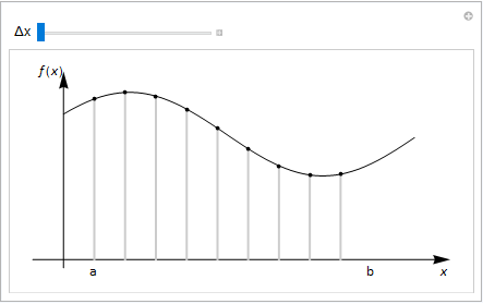
Fig. 6.5 The average of a discrete function is given by adding up the values and dividing by the number of points. We extend this concept to continuous functions in the limit as \(\Delta x\rightarrow 0\).

As shown in Fig. 6.5, for any function \(f(x)\) we can obtain the average output \(\bar{f(x)}\) by adding up a series of outputs and dividing by the number of datapoints used. In this case, the spacing between datapoints is \(\Delta x\). By taking the limit as \(\Delta x\rightarrow 0\) we can obtain:

(6.7)\[\bar{f} = \frac{1}{n}\displaystyle \sum_{j=0}^{n-1}f(x_j) = \frac{\Delta x}{b-a}\sum_{j=0}^{n-1}f(x_j) \rightarrow \frac{1}{b-a}\displaystyle \int_a^b f(x)\mathrm{d}x\]

Example

Calculate the mean value of \(\cos ^3(\theta)\) on the interval \(\left[-\frac{\pi}{3}, \frac{\pi}{3}\right]\) by integration.

Solution

\(\frac{1}{\frac{\pi}{3} - \left(-\frac{\pi}{3}\right)}\displaystyle \int_{-\pi/3}^{\pi/3}\cos^{3}(\theta)\mathrm{d}\theta = \frac{3}{2\pi}\displaystyle \int_{-\pi/3}^{\pi/3}\cos(\theta)(1-\sin^2(\theta))\mathrm{d}\theta\)

\(=\frac{3}{2\pi}\left[\sin(\theta)-\frac{1}{3}\sin^3(\theta)\right]_{-\pi/3}^{\pi/3} = \frac{9\sqrt{3}}{8\pi}\)

6.3.2. Arc Length

Fig. 6.6 illustrates how the length of an arc along a curve \(y(x)\) betwenn \(x=a\) and \(x=b\) can be computed by adding togather individual segments.

Fig. 6.7 shows how each contribution of \(\Delta s\) from the length of each segment is calculated.

Then by summing these lengths in the limit as \(\Delta x \rightarrow 0\), we obtain the following formula for arc length:

(6.8)\[L = \displaystyle \int_a^b \sqrt{1+\left(\frac{\mathrm{d}y}{\mathrm{d}x}\right)^2}\mathrm{d}x\]

For a curve given parametrically in the manner \(x(t)\), \(y(t)\), we have:

(6.9)\[\begin{split}\frac{\mathrm{d}y}{\mathrm{d}x} = \frac{\mathrm{d}y}{\mathrm{d}t}\biggr/\frac{\mathrm{d}x}{\mathrm{d}t} = \frac{\mathrm{d}y}{\mathrm{d}t}\frac{\mathrm{d}t}{\mathrm{d}x} \\ \textrm{which gives} \\ L=\displaystyle \int_{t_0}^{t_1}\sqrt{\left(\frac{\mathrm{d}x}{\mathrm{d}t}\right)^2+\left(\frac{\mathrm{d}y}{\mathrm{d}t}\right)^2}\mathrm{d}t\end{split}\]

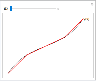
Fig. 6.6 To estimate the arc length along a curve, we can add together segments as shown. By decreasing the difference \(\Delta x\) between the joined up points, we obtain a better approximation.

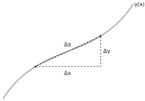
Fig. 6.7 The distance \(\Delta s\) moved along a curve, corresponding to small changes \(\Delta x \Delta y\) can be calculated by Pythagoras’ formula as \(\Delta s = \sqrt{\Delta x^2 + \Delta y^2} = \sqrt{1+\left(\frac{\Delta y}{\Delta x}\right)^2}\Delta x\)

Example

Example 1

Find the length of the arc of the curve \(x = 18t^2\), \(y=(12t+9)^\frac{3}{2}\) from \((0,27)\) to \((32, 125)\).

Solution 1

We have:

\(\frac{\mathrm{d}x}{\mathrm{d}t}=36t\), \(\frac{\mathrm{d}y}{\mathrm{d}t}=\frac{3}{2} (12)(12t+9)^{1/2}=18(12t+9)^{1/2}\)

Then, as all lenths are positive:

\(L = \displaystyle \displaystyle \int_{t=0}^{4/3}\sqrt{(36t)^2+18^2(12t+9)}\mathrm{d}t = 18\displaystyle \int_{0}^{4/3}\sqrt{(3+2t)^2}\mathrm{d}t = 18\displaystyle \int_0^{4/3}(2t+3)\mathrm{d}t\)

Thus:

\(L=18\biggr[t^2+3t\biggr]_0^{4/3}=104\) units.

Example 2

Calculate the arc length of the curve defined by \(x=\cos(t)\), \(y=\sin(t)\), between \(t=\frac{\pi}{6}\) and \(t=\frac{\pi}{3}\).

Solution 2

\(\displaystyle \int_{\pi/6}^{\pi/3}\sqrt{\left(\frac{\mathrm{d}x}{\mathrm{d}t}\right)^2+\left(\frac{\mathrm{d}y}{\mathrm{d}t}\right)^2}\mathrm{d}t =\displaystyle \int_{\pi/6}^{\pi/3}\sqrt{\sin^2(t)+\cos^2(t)}\mathrm{d}t =\left[t\right]_{\pi/6}^{\pi/3}=\frac{\pi}{6}\)

The result simply gives the arc length of a portion of the unit circle (\(x^2 + y^2 = 1\)) between \(\theta=\frac{\pi}{6}\) and \(\theta=\frac{\pi}{3}\)

Example 3

Calculate the length of the curve \(y=2(x-1)^\frac{3}{2}\) between \(x=1\) and \(x=4\).

Solution 3

\(\frac{\mathrm{d}y}{\mathrm{d}x}=3\sqrt{x-1}\)

\(\mathrm{d}S=\sqrt{1+\left(\frac{\mathrm{d}y}{\mathrm{d}x}\right)^2}\mathrm{d}x=\sqrt{1+9(x-1)}\mathrm{d}x=\sqrt{9x-8}\mathrm{d}x\)

\(S=\displaystyle \int_{x=1}^{x=4}\sqrt{9x-8}\mathrm{d}x = \displaystyle \int_1^4(9x-8)^{1/2}\mathrm{d}x = \left[\frac{2}{27}(9x-8)^{3/2}\right]_1^4 = \frac{2}{27}(56\sqrt{7}-1)\)

6.3.3. Surface area and volume of revolution

Fig. 6.8 shows how a surface can be obtained from rotating a curve about an axis.

To calculate the area of the surface:

Point \(y(x)\) is rotated about the horizontal axis, giving circumference \(2\pi y\). Then we integrate along the surface (along a segment of arc \(\Delta s\) in the limit \(\Delta s\rightarrow 0\))

(6.10)\[A = \displaystyle \int_a^b 2\pi y\mathrm{d}s = \displaystyle \int_a^b 2\pi y\sqrt{1+\biggr(\frac{\mathrm{d}y}{\mathrm{d}x}\biggr)^2}\mathrm{d}x\]

To calculate the volume, we add up cylindrical “slices” \(\pi ^2 \Delta x\) in the limit as \(\Delta x \rightarrow 0\):

(6.11)\[V = \displaystyle \int_a^b \pi y^2 \mathrm{d}x\]

Note

Instead of using cylindrical slices, we could use “frustrums” (sections of cones). The result would be the same (in the limit \(\Delta x \rightarrow 0\)).

Similarly, when calculating the area under the curve, we used rectangles, but we could have used parallelograms.

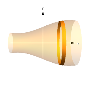
Fig. 6.8 Rotating an arc length \(\Delta s\) about the \(x\)-axis produces an approximately cylindrical surface with area \(\Delta A = 2\pi y \Delta s\).

Example

Prove by integration that the curved area of the cone is \(\pi r \lambda\), where \(\lambda\) is the slant length (as shown in Fig. 6.9).

What is the volume of this cone?

Solution

Rotate the line \(y=\frac{r x}{h}\) about the \(x\)-axis to give:

\(S=\displaystyle \int_0^h 2\pi \frac{rx}{h}\sqrt{1+\left(\frac{r}{h}\right)^2}\mathrm{d}x = \frac{2\pi r}{h^2}\sqrt{h^2+r^2}\displaystyle \int_0^h x\mathrm{d}x = \pi r\sqrt{h^2+r^2}=\pi r \lambda\)

The volume is given by:

\(V=\displaystyle \int_0^h\pi\left(\frac{rx}{h}\right)^2\mathrm{d}x = \pi\frac{r^2}{h^2}\biggr[\frac{x^3}{3}\biggr]_0^h = \pi \frac{r^2}{3}h\)

This is as expected, as it is equivalent to \(\frac{1}{3} \cdot base \cdot height\).

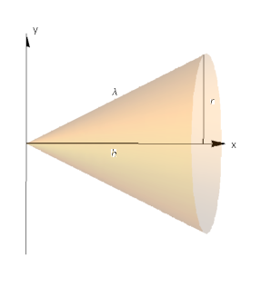
Fig. 6.9 Depiction of a cone, as mentioned in the above example.

5. Differentiation 7. Taylor series