7. Taylor series
7.1. Taylor expansion definition
We will write the formula for expansion about \(x=a\), in which we seek to express \(f(x)\) as an infinite polynomial of the form
We choose the coefficients \(c_n\) to ensure that the \(n^{\text{th}}\) derivative of the polynomial is equal to the \(n^{\text{th}}\) derivative of the function at the point \(x=a\). In this sense, the Taylor series gives the best possible local polynomial approximation to \(f(x)\) of specified degree.
By repeatedly differentiating and evaluating the polynomial, we obtain
This result defines the Taylor series for \(f(x)\), given in the box below.
Taylor series for \(f(x)\) about a point \(x=a\).
The special case when \(a=0\) is known as the Maclaurin series for historical reasons.
An important example: Taylor expansion of \(f(x)=e^x\) about \(x=0\)
\(f'(x)=e^x,\ f''(x)=e^x\ ...,\) so
Notice that this series satisfies \(\frac{\mathrm{d}p}{\mathrm{d}x}=p\).
More important examples:
The Maclaurin expansions of \(\sin\), \(\cos\), \(e^x\), and \(\ln(1+x)\) are particularly important:
\(\displaystyle \sin(x) = x-\frac{x^3}{3!}+\frac{x^5}{5!}-\dots+ = \sum_{n=0}^{\infty}\frac{(-1)^n x^{2n+1}}{(2n)!}\)
\(\displaystyle \cos(x) = 1-\frac{x^2}{2!}+\frac{x^4}{4!}-\dots+ = \sum_{n=0}^{\infty}\frac{(-1)^n x^{2n}}{(2n)!}\)
\(\displaystyle e^x = 1+x+\frac{x^2}{2!}+\dots+ = \sum_{n=0}^{\infty}\frac{x^n}{n!}\)
\(\displaystyle \ln(1+x) = x-\frac{x^2}{2}+\frac{x^3}{3}-\dots+ = \sum_{n=0}^{\infty}\frac{(-1)^n x^{n+1}}{n+1}\)
You should also be able to calculate the first few terms in the expansion of an arbitrary function \(f(x)\).
Exercise:
By regrouping the terms in the Maclaurin series for \(e^{i\theta}\), derive Euler’s formula.
Solution :
We can write this out rigorously as follows:
A disclaimer!
Not all functions are faithfully represented by their Taylor Series. We have only guaranteed that the polynomial has the “correct” behaviour in the immediate vicinity of the point \(x=a\). Two things should be checked:
Does the series converge to a finite value for all \(x\)?
If not then it is important to find the radius of convergence. This can be achieved by using the ratio testDoes it converge to \(f(x)\)?
Even if the series converges, there is no guarantee that it converges to \(f(x)\).
We would need to show that \(\displaystyle \lim_{k\rightarrow \infty}|f(x)-p_k(x;a)|=0\), which may only be true for some values of \(x\).
This can be done by making use of the Lagrange remainder theorem, introduced in the next subsection.
Functions which converge to their Taylor series for a range of values are called analytic, and functions which converge to their Taylor series everywhere are called entire. The sine and cosine series, and the \(e^x\) series are entire. The Maclaurin series for \(\ln(1+x)\) is analytic for \(|x|<1\).
7.1.1. Practical use
The Taylor series nearly always contains an infinite number of terms. To be of practical use in applications, we typically need to “truncate” the expansion, meaning that we retain only the terms up to a specified \(n^{\text{th}}\) power of \(x\).
Example: The two-term expansion
Let us examine what happens if we retain just the first two terms in the Taylor series:
This defines a straight line.
The line passes through the point \((a, f(a))\) so it touches the curve f(x) at the point \(x = a\)
The line has slope \(f^{\prime}(a)\), which is the gradient of the curve at \(x = a\)
Therefore, the two-term Taylor series is just the tangent to the curve!
The tangent is the best possible approximation that we can obtain for the curve near the point \(x = a\) using only two terms.
As well as considering the validity of the infinite series, it is important to be able to determine how many terms in the series are needed for practical use. If the series converges very slowly, then it may not be much good!
As can be seen from the plot below, the degree 21 Maclaurin expansion \(\sin(x)\) already represents \(\sin(x)\) rather faithfully on the range \([-2\pi,2\pi]\), but it is less accurate further away from the expansion point.
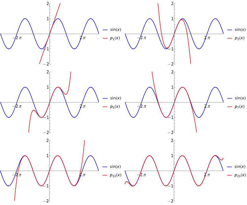
Fig. 7.1 A plot of the curve \(\sin(x)\) together with Maclaurin series expansion retaining successively greater numbers of terms, \(p_1,p_3,p_5,p_7,p_{13},p_{21}\).
7.1.2. Advanced: Lagrange remainder theorem
The Lagrange remainder theorem, given in the box below, allows us to place precise bounds on the size of the error. The result shows that the error in the truncated expansion is proportional to the next power of \((x-a)\).
Lagrange remainder theorem
Let \(p_n(x;a)\) be the truncated Taylor expansion of \(f(x)\) about point \(x=a\), up to and including the term in \((x-a)^n\). The remainder (error) in the truncated expansion is given by
We say that the degree \(n\) series has “order \((x-a)^n\) accuracy”, and we may write
where the big-O notation describes the order of the error terms.
The power-relationship in Lagrange’s theorem can be anticipated when \((x-a)\) is small, and for larger differences by noting that the factorial growth of the coefficient denominators is much faster than polynomial growth.
Big idea : Local approximation of a function
We can compute a series expansion for a function in powers of \(x\) using Taylor series. The resulting truncated polynomial gives a good local approximation to a function in a sense made precise by the Lagrange remainder theorem. If the truncated polynomial is used near the expansion point \(a\) then its accuracy “goes like” the \(n^{\text{th}}\) power of the distance from \(a\).
The proof of the Lagrange remainder theorem, and derivation of the coefficient of \((x-a)^n\) is found by using another result called the mean value theorem. It won’t be of much benefit for our practical purposes to show the proof here. Instead, let us take a look at an illustrative example.
Example
Use the Lagrange remainder theorem to compute an upper bound for the size of the error in the quadratic expansion of \(\sin(x)\) about \(x=\frac{\pi}{3}\), at a nearby point \(x=\frac{\pi}{2}\).
Solution
The series expansion is found to be:
And from Lagrange’s formula, the error in the expansion at \(x=\frac{\pi}{2}\) is given by
Since \(|\cos(\xi)|\) is bounded above by \(1\) on the given domain, Lagrange’s remainder theorem gives an upper bound of \(\frac{\pi^3}{6^4}=0.0239246\) The exact error is
7.1.3. Advanced: Composite function expanions
Let \(P(x)\), \(Q(x)\), be two power series that converge to \(f(x)\) and \(g(x)\) respectively Then
\(aP(x) + bQ(x)\) converges to \(af(x)+ bg(x)\)
\( P(x)Q(x)\) converges to \(f(x)g(x)\)
\( P(Q(x))\) converges to \(f(g(x))\)
It means that we can construct the Taylor series for a composite function by using known results for elementary functions (although we need to take care to check the region of validity)
Example 1 :
\(e^{\sin(x)}=1+\sin(x)+\frac{\sin(x)^2}{2!}+{\sin(x)^3}{3!}+...\) \(=1+(x-\frac{x^3}{3!+...})+\frac{1}{2!}(x-\frac{x^3}{3!+...})^2+\frac{1}{2!}(x-\frac{x^3}{3!+...})^3+.... =1+x+\frac{1}{2!}x^2+0x^3+...\)
This is valid everywhere since the series expansions for both \(\sin\) and \(\exp\) are entire)
Example 2 :
Find The Maclaurin series for \(\ln(\frac{1+x}{1-x})\), and determine the interval of convergence for this expansion
Solution :
The series expansion of \(\ln(1+x)\) can be found by taking \(f(x)=\ln(1+x)\) in the general formula, about the point \(x=0\).
We can use the result to obtain:
\(\ln\left(\frac{1+x}{1-x}\right) = \ln(1+x)-\ln(1-x) = \left(x-\frac{x^2}{2}+\frac{x^3}{3}-\frac{x^4}{4}+\frac{x^5}{5}-\dots\right) - \left(-x-\frac{x^2}{2}-\frac{x^3}{3}-\frac{x^4}{4}-\dots\right)\)
\(\displaystyle =2x+\frac{2x^3}{3}+\frac{2x^5}{5}+\dots = \sum_{n=1}^{\infty}\frac{2x^{2n-1}}{2n-1}\)
To find the radius of convergence, we let \(u_{n} = \frac{2x^{2n-1}}{2n-1}\). Then,
\(\displaystyle\lim_{n\rightarrow\infty}\frac{u_{n+1}}{u_n} = x^2\lim_{n\rightarrow\infty}\left(\frac{2-\frac{1}{n}}{2+\frac{1}{n}}\right)=x^2\)
The series converges for \(-1<x<1\).
When \(x=\pm 1\), the series expansion is equal to \(\pm 2(1+\frac{1}{3}+\frac{1}{5}+\frac{1}{7}+\dots)\), which does not converge. For these values of \(x\), the function \(f(x)\) is also not finite.
7.1.4. Application: L’Hôpital’s Rule
A tricky, yet common, problem involves finding the limit of a ratio of two functions that both approach zero.
For example, what is the value of the following limit?
Trying some small values of \(x\) on a calculator suggests that the result approaches 1, but can we prove it analytically?
Note: we also need to take care when dividing, multiplying or subtracting small values or values which differ by a small amount on a calculator. Numeric rounding errors can lead to very badly behaved results!
To prove the result analytically, we use the series expansion for sine:
A general result based on this type of approach is given in the box below.
L’Hôpital’s rule :
If \(\displaystyle \lim_{x\rightarrow c}f(x)=\lim_{x\rightarrow c}g(x)=0\) then
(provided both these limits exist and are finite)
Extended L’Hôpital’s rule :
If \(\displaystyle \lim_{x\rightarrow c}f(x)=\lim_{x\rightarrow c}g(x)=\infty\) then
(provided both these limits exist and are finite)
We can apply these results repeatedly
Proof:
\(\displaystyle \lim_{x\rightarrow c}\frac{f(x)}{g(x)}=\lim_{x\rightarrow c}\frac{f(c)+f^{\prime}(c)(x-c)+\dots}{g(c)+g^{\prime}(c)(x-c)+\dots}\)
Since we are taking the limit as \(x\rightarrow c\) we are guaranteed that the Taylor series approximation is faithful if the function is differentiable.
Example 1 :
Determine, with justification, the value of the limit
\(\displaystyle \lim_{x\rightarrow 0}{\left(\frac{\sin^2(x)}{3 x^2 + 2x}\right)}\)
Solution :
\(\displaystyle \lim_{x\rightarrow 0}{\left(\frac{\sin^2(x)}{3 x^2 + 2x}\right)}=\displaystyle \lim_{x\rightarrow 0}{\left(\frac{2\sin(x)\cos(x)}{6x+2}\right)}=0\)
Example 2 :
\(\displaystyle\lim_{x\rightarrow\infty}x^2 e^{-x}=\lim_{x\rightarrow\infty}\frac{x^2}{e^x}=\lim_{x\rightarrow\infty}\frac{f(x)}{g(x)}\)
where \(f(x)=x^2\), \(g(x)=e^x\) and both functions approach \(\infty\) in the limit.
Solution :
\(f^{\prime}(x)=2x\) so \(f^{\prime}(\infty)=\infty\)
\(g^{\prime}(x)=e^x\) so \(g^{\prime}(\infty)=\infty\)
\(f^{\prime\prime} (x)=2\)
\(g^{\prime\prime}(x)=e^x\)
\(\displaystyle \lim_{x\rightarrow\infty} x^2 e^{-x} = \lim_{x\rightarrow\infty}\frac{2}{e^x}=0\)