1. Limits of Functions and Sequences
The mathematics of limits is used to describe the behaviour of a function or sequence that is not AT a point, but approaching it.
The limits of a function are best illustrated by example.
1.1. Example: \(f(x) = x^2\)
We start with a trivial example, by considering the function \(f(x) = x^2\) near to the point (2,4).
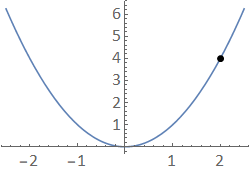
Fig. 1.1 A plot of \(f(x)=x^2\) together with the point \((2,4)\).
In this example, it is apparent that we can trace along the \(x^2\) curve towards the point, from either direction. Mathematically, we say that we can make \(f(x)\) arbitrarily close (“as close as you like”) to 4 by making \(x\) sufficiently close to 2. We write
and we say that “the limit of \(x^2\) as \(x\) tends to (approaches) 2 is equal to 4”. In fact, for the squared function, it is clear that
for all \(c\). However we will see that this behaviour does not apply for all functions.
We may also consider the limit of a function \(f(x)\) as its argument \(x\) becomes “very large”. For instance, we can say that \(\displaystyle\lim_{x\to\infty} x^2 = \infty\) since \(x^2\) can be made arbitrarily large by making \(x\) “big enough”. For instance, we can make \(x^2\) larger than \(10^{998}\) by making \(x\) larger than \(10^{499}\).
We would read the expression by saying: “the limit of \(x^2\) as \(x\) tends to infinity is infinity”, though it does not actually reach infinity.
1.2. Example: \(f(x) = \frac{1}{x}\)
Whilst the limit of \(x^2\) for large \(x\) is non-finite, there are other functions which approach a finite value as \(x \to \infty\), and also functions which approach a non-finite value whilst \(x\) remains finite. For example, consider the behaviour of \(f(x) = \frac{1}{x}\), illustrated in the plot below.
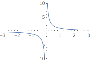
Fig. 1.2 A plot of \(f(x)= \frac{1}{x}\).
In this case, as \(x\) becomes very large, \(f(x)\) approaches zero. We write that
The \(0^+\) and \(0^−\) have been used here to indicate that the function “tends to zero from above/below” as \(x\) tends to positive and negative infinity respectively.
Near to \(x=0\), the behaviour of \(\frac{1}{x}\) is different to what we have seen so far:
As \(x\) tends to zero from above (from the right), the graph shoots off to positive infinity, but…
As \(x\) tends to zero from below (from the left), the graph shoot off to negative infinity.
1.3. The one-sided limit
The previous example motivates the idea of a one-sided limit. We write that
Since the left- and right- limits are not the same, then we cannot meaningfully refer to “the limit” without providing a direction, so the result for \(\displaystyle\lim_{x \to 0} \frac{1}{x}\) is undefined. We say that the function is discontinuous at \(x = 0\), though it is “piecewise continuous” on each of the pieces either side of \(x=0\).
Another example of a piecewise continous function is the Heaviside function, which we define as:
although it may be defined otherwise (e.g. with \(H(0)=\frac{1}{2}\)). A plot of this function is shown below. It has a finite jump discontinuity at \(x=0\).
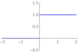
Fig. 1.3 A plot of the Heaviside function \(H(x)\).
1.4. Combination of limits
It is useful to know how to solve the limit of combinations of functions (or so called functions of functions) such as
where \(c\) will can be any number such as \(0\), \(1\) or \(\infty\).
The approach we take to solve these depends on whether the limits of the inidividual functions \(\displaystyle\lim_{x \to c} f(x)\) and \(\displaystyle\lim_{x \to c} g(x)\) are finite or infinite.
1.4.1. Functions that tend to finite values
First consider the case where the limit of all the functions are finite. If and only if the limits of the individual functions are FINITE then we can use the combination theorem to solve the combination of functions.
The combination theorem for limits
If the limits \(\displaystyle\lim_{x \to c} f(x)\) and \(\displaystyle\lim_{x \to c} g(x)\) are finite then,
where \(\alpha\) and \(\beta\) are constants. To stress the point again, the combination theorem for limits can only be used if the limit of every function is finite.
As an example, consider the function:
Since the limits of each of the individual functions are finite: \(\displaystyle\lim_{x \to 0} x^2 = 0\), \(\displaystyle\lim_{x \to 0} (x+1)^3 = 1\) and \(\displaystyle\lim_{x \to 0} (x-1)^3 = -1\), we can use first and third statment of the combination theorem to rewrite and solve the equation as:
So we can conclude the limit of the function is \(0\).
1.4.2. Functions that tend to infinite values
We now consider the case where the limit of all the individual functions are infinite, such as \(\displaystyle\lim_{x\to \infty} x^2 = \infty\) and \(\displaystyle\lim_{x\to 0^-} \frac{1}{x} = -\infty\).
The approach we take can be illustrated by the following two examples:
Example 1
This limit appears to “go like” \(\infty - \infty\), so you would be forgiven for thinking this result is zero. On the other hand, there is a sense in which \(x^2\) is “much bigger” than \(x\) and so it dominates this expression. That is \(x^2\) “blows up faster” than \(x\) as \(x\to \infty\). Indeed, if you try subsitute a large value of \(x\) into the function \((x^2 - x)\) you may infer that function can get arbitrarily large by making \(x\) sufficiently large. So this limit appears to be infinity.
Another way to approach this problem is to factorise \((x^2 - x) = x (x-1)\); both \(x \to \infty\) and \(x-1 \to \infty\) as \(x\to\infty\).
Example 2
The second limit “goes like” \(\frac{\infty}{\infty}\), but the answer is not one. To solve this limit we consider the behaviour of the numerator and denominator separately. We note that the function \(x\) is “much much” greater than \(\sqrt{x + 2}\) for large \(x\) (i.e. \(x >> \sqrt{x + 2}\)) so we say that the numerator “goes like” \(x\) for large \(x\). The denominator simply “goes like” 4𝑥, so the fraction in the limit “goes like” \( \frac{x}{4 x} = \frac{1}{4}\). Again, you may convince yourself of this by taking some large values of \(x\) on your calculator - though note that your calculator may not be able to handle the ratio if you make the values too large.
Another approach you may take is to simplify the function first:
Because \(\displaystyle\lim_{x\to\infty} \frac{1}{x} = \lim_{x\to\infty} \frac{2}{x^2} = 0\), we can see we also arrive at the solution of \(\frac{1}{4}\). As an exercise, convince yourself of the following result:
Summary
From the 2 examples above we illustrate that the solutions can be found be determining the individual function(s) (which may be constant values) that dominate in the limit. It most cases it is useful to simply the equation before tackling the limit.
It must be noted that fractions which “go like” \(\frac{\infty}{\infty}\) do not necessarily approach a finite limit. For instance, the result \(\displaystyle\lim_{x \to \infty} \frac{x+2}{x^2 - x}\) is equal to zero, since the degree of the denominator is larger than the degree of the numerator and it dominates. That is, the denomiator “blows up faster” than the numerator.
1.4.3. Questions
Find the following limits:
\(\displaystyle\lim_{x\to\infty} \frac{x+2}{x^2-2}\).
\(\displaystyle\lim_{x\to\infty} \frac{x-2}{x+2}\).
\(\displaystyle\lim_{x \to \infty} \big( \sqrt{x^2-2} - \sqrt{x^2+x} \big)\).
Solutions
\(\displaystyle\lim_{x \to \infty}\frac{x+2}{x^2 - 2} = \lim_{x \to \infty} \frac{1/x + 2/x^2}{1-2/x^2}\) \(= \frac{0+0}{1+0}\) \(=0\).
\(\displaystyle\lim_{x \to \infty}\frac{x-2}{x+2} = \lim_{x \to \infty} \frac{1 - 2/x}{1+2/x}\) \(= \frac{1-0}{1+0}\) \(=1\).
\(\sqrt{x^2-2} - \sqrt{x^2+x}\) \( = \big(\sqrt{x^2-2} - \sqrt{x^2+x} \big) \frac{\sqrt{x^2-2} + \sqrt{x^2+x}}{\sqrt{x^2-2} + \sqrt{x^2+x}}\) \( = \frac{-x-2}{\sqrt{x^2-2} + \sqrt{x^2+x}}\) \( = \frac{-1-2/x}{\sqrt{1-2/x^2} + \sqrt{1+1/x} }\). Thus, \(\displaystyle\lim_{x \to \infty} \big(\sqrt{x^2-2} - \sqrt{x^2+x} \big)\) \(= \frac{-1-0}{1+1}\) \( = -\frac{1}{2}\).
1.5. Sequences
Your intuition of a sequence will likely be correct. It can mean a sequence of letters, such as a word (e.g. A, U, S, T, R, A, L, I, A) or a DNA sequence (e.g. A, T, T, C, G, G, T, C, A, T, C). It can also be a sequence of numbers such as a telephone number, date of birth, something nonsensical (e.g. \(181291, 2, -4309, \sqrt{7}\)) or the prime numbers: \(2, 3, 5, 7, 11, \dots\). Here, the dots indicate that the sequence goes on infinitely.
Each part of the sequence is called a term. Each sequence has a specific ordering of terms. For example, the series \(1,2,3,4\) is different from the series \(4,3,2,1\) much in the same way that the telephone number \(18001234\) will reach a different person to the phone number \(18004321\).
1.5.1. Definition
Sequence
A sequence is a set of terms where order matters, written as follows:
Here, the size of the sequence (the number of terms) is \(n\). The \(i\)-th term in the sequence may be denoted by \(u_i\) where \(i = 1, 2, \dots, n\).
The labels \(u\), and \(i\) are arbitrary, and we could just as well use other letters to represent them. Sequences can have finite \(n<\infty\) (e.g. telephone numbers) or infinite sizes \(n \to \infty\) (e.g. the prime numbers).
The sequences that we will examine in this course are numerical patterns. Much of mathematics is concerned with patterns in both mathematical constructs and nature, and the study of sequences provides a firm grounding for this endeavour.
Mathematical patterns can generally be expressed as formula for the \(i\)th term. For instance, the formula below generates the sequence \(-1, 2, 5, 8, 11, 14, 17, 20\) by taking \(i=1,\dots 8\) :
Notice that the size of the terms in this sequence grows without bound as the number of terms is increased.
1.5.2. Recurrence relationships
It is sometimes possible to express a sequence as a formula, otherwise known as a recurrence relation, which sets out the rule(s) to find the sequence.
A famous example
A well-know example that arises in many natural systems is the Fibonacci sequence:
This sequence is generated by starting with the sequence \(0,1\) and finding the next number in the sequence by adding the two previous numbers together, e.g. \(0+1=\mathbf{1}\), \(1+1=\mathbf{2}\), \(1+2=\mathbf{3}\), \(2+3=\mathbf{5}\), \(3+5=\mathbf{8}\), etc.
The sequence can be expressed as the formula
which specifies the \(i\)-th term provided we have the term for \(i-1\) and \(i-2\). It is because of this formula that it is necessary to provide the first two terms of the sequence, \(u_1=0\) and \(u_2=1\), to find the rest of the sequence.
Python code for Fibonacci sequence:
nterms = 10 # number of terms
u1, u2 = 0, 1 # first two values
count = 0 # counter
while count < nterms: # while loop
       print(u1) # print values
       nth = u1 + u2 # recurrence relation
       u1 = u2 # update values
       u2 = nth # update values
       count += 1 # update counter
You can use this webpage to run basic python scripts.
Note that the Fibonnaci recurrence relation will generate a different sequence to the Fibonacci sequence when the starting terms are different (e.g. \(u_1=10\) and \(u_2=11\)).
Exercise
Convince yourself that the formula \(u_i = 2 + u_{i-1}\) provides the sequence of even numbers when
\(u_1=2\) and the sequence of odd numbers when \(u_1=1\).
Python code for even numbers:
nterms = 10 # number of terms
u = 0 # first value
count = 0 # counter
while count < nterms: # while loop
       print(u) # print values
       u = u + 2 # recurrence relation
       count += 1 # update counter
Can you edit this code to produce the sequence of odd numbers?
Recurrence relations, although simple, can produce surprisingly complicated behaviours. For further reading you may like to study the logistic map:
where \(r\) is a constant. This equation (which models animal population growth) opened up the field of chaos theory.
1.5.3. Limits of sequences
In what comes next, we will be interested in calculating the “limit” of (i) the terms in a sequence \(u_k\) as \(k \to \infty\), and (ii) the value of a function \(f(x)\) as \(x \to c\) where \(c\) can be a finite or infinite number.
We may distinguish the cases where:
the function and terms in a sequence diverge to an infinite value (blow up to \(\pm \infty\)),
the function and terms in a sequence converge to a finite value.
Link to a video introducing the concept of a limit.
1.5.3.1. Definition
The limit of a sequence is the value that the terms of a sequence approaches (or tends to) as the number of terms approaches infinity, written as \(k \to \infty\) if \(k\) were the index variable.
The limit of a sequence
For a sequence \((u_1, u_2, u_3, \dots)\), the limit of a sequence is written as
We say that a number, say \(U\), is the limit of a the sequence \((u_1, u_2, u_3, \dots)\) if the numbers of the sequence \(u_k\) approach \(U\) as \(k\to\infty\). We say that the limit of the sequence diverges if \(\lvert U \rvert =\infty\) and converges if \(\lvert U \rvert < \infty\).
1.5.3.2. Similarity to limits of a function
It is important to note that similarity between the limits of a sequence and a function. A function \(f(x)\) for real number \(x\) will have the same limit as the sequence \(u_k = f(k)\) for integer number \(k\). For example \(f(x) = x^2\), the limit \(\displaystyle\lim_{x \to \infty} f(x) = \infty\) is the same as the limit (infinite) of the sequence with terms \(u_k = k^2\), \((1, 2, 4, 16, \dots)\).
The key difference is that when we refer to the limit of a sequence we always mean the limit of the terms \(u_k\) as the numbers of terms go to infinity \(k\to\infty\). This is not the case for the limit of functions where the variable (i.e. \(x\)) can go to any number.
Consider another example from the previous section, the limit of the infinite sequence with terms \(u_k = \frac{1}{k}\) for \(k=1,2,\dots\):
is \(0\) in the same way that the limit of the functon \(\frac{1}{x}\) is zero, \(\displaystyle \lim_{x\to\infty} \frac{1}{x} = 0\).