11. ODEs with Python
## preamble : This part loads the packages that we will use

import numpy as np                   #for linspace
from scipy.integrate import odeint   #for odeint
import matplotlib.pyplot as plt      #for plotting
We will use the “odeinit” package, which is designed to solve problems of the form
where \(X\) is a list of dependent variables and c is a sequence of parameters.
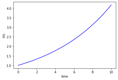
11.1. Example 1: Exponential growth
The first step requires us to set up a function that returns the derivative for a given value of \(I\), and parameters \(\mu,r_0\).
In the code below, notice that \(t\) appears as the second input argument even though it doesn’t feature explicitly on the RHS of the equation. This is because the odeint solver expects a function pattern \(f(X,t,c)\).
# Model definition
def dIdt(I,t,mu,r0):
  return mu*(r0-1)*I
You can test the definition, by plugging in some values of \(\mu,r_0,I\) and printing the result. You will have to supply a value for \(t\) as well, but since there is no dependence on this variable it won’t affect the result. I’ve taken \(t=1\).
# Taking I=2, t=1, mu=1/14, r0=3:
print(dIdt(2,1,1/14,3))
0.2857142857142857
Now we will use the function that we created to find a numeric estimate of the ODE solution between \(t=0\) and \(t=10\).
Since we are using a numeric solver, we will need to provide an initial condition for \(t(0)\). The numeric algorithm will then solve the equations of motion at discrete time steps, by treating the derivatives as constant over a small interval. We will split up the time domain into a list of equally spaced points by using the linspace function from the numpy package.
This is an approximation, so it won’t give a totally accurate result, but it will usually be a good estimate if the time steps are small enough.
Recall that the mathematical definition of the derivative actually requires bringing the points together, in the limit
I0 = 1                       # initial condition

n,tmax = 401,10              # n is number of time points
t = np.linspace(0,tmax,n)    # time points

# solve ODE
I = odeint(dIdt,I0,t,args=(1/14,3))

# plot results
plt.plot(t,I,'b-')
plt.ylabel('I(t)')
plt.xlabel('time')
plt.show()
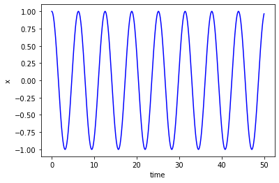
11.2. Example 2: Simple Harmonic Motion
The SHM equation is
where \(k,m\) are parameters. The problem can be written in the required form by defining \(y=\dot{x}\) to give
We will set up a function that returns this derivative for given values of \(X=(x,y)\), and parameters \(k,m\).
Notice that we use \(X[0],X[1]\) for \(x,y\).
This is because Python indexing starts from zero, so \(X[0]\) is the first element obtained from the list \(X=(x,y)\).
# Model definition
def dXdt(X,t,k,m):
  dxdt = X[1]          #dx/dt = y
  dydt = -k*X[0]/m     #dy/dt=-k*x/m
  return [dxdt, dydt]
For example, suppose that the system starts from rest at \(x(0)=1\), \(\dot{x}(0)=0\).
Taking the constants to be \(k=m=1\) gives the following result for \(\frac{\mathrm{d}X}{\mathrm{d}t}\) at time \(t=0\):
t0,X0 =0,[1,0] #initial conditions for t,x,y
k,m = 1,1
X = dXdt(X0,t0,k,m)
print(X)
[0, -1.0]
Now we will use the function that we created to find a numeric estimate of the solution between \(t=0\) and \(t=100\).
The odeint function will return the numeric estimates for \(x,y\) at the corresponding time points, as columns in an array.
We can access the first column by using \(X[:,0]\) and the second column by using \(X[:,1]\)
tmax,n=50,1000
t = np.linspace(t0,tmax,n)    # time points

# solve ODE
X = odeint(dXdt,X0,t,args=(k,m))

# plot results
plt.plot(t,X[:,0],'b')
plt.ylabel('x')
plt.xlabel('time')
plt.show()
11.3. Example 3: SHM with forcing
Now let’s see what happens if we add in a forcing term
where \(F=1\), and \(\Omega=1.1\) :
# Re-define the model to include the forcing term
def dXdt(X,t,k,m,F,W):
  dxdt = X[1]                          #dx/dt = y
  dydt = -k*X[0]/m + F*np.sin(W*t)     #dy/dt=-k*x/m + F*sin(W*t)
  return [dxdt, dydt]

t0,X0 =0,[1,0] #initial conditions for t,x,y
k,m,F,W = 1,1,1,1.1

tmax,n=200,1000
t = np.linspace(t0,tmax,n)    # time points

# solve ODE
X = odeint(dXdt,X0,t,args=(k,m,F,W))

# plot results
plt.plot(t,X[:,0],'b')
plt.ylabel('x')
plt.xlabel('time')
plt.show()
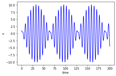
Experiment with making \(\Omega\) closer to \(1\). What happens?
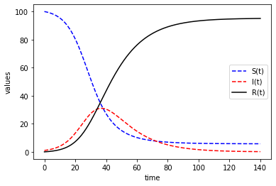
11.4. Example 4 : The SIR model of infection
In this model, \(S\) represents people who are susceptible to catching an infection, \(I\) represents people who already have the infection, and \(R\) represents people who have recovered.
We will solve the model between \(t=0\) to \(t=140\), taking \(\mu=1/14\), \(\beta=3/14\), \(N=100\).
# Model definition
def dXdt(X,t,mu,beta,N):
  dSdt= -beta*X[0]*X[1]/N
  dIdt= beta*X[0]*X[1]/N - mu*X[1]
  dRdt= mu*X[1]
  return [dSdt,dIdt,dRdt]

pop = 100       # population size
X0 = [pop,1,0]  # initial condition

# solve ODE
tmax,n = 140,401
t = np.linspace(0,tmax,n)
X = odeint(dXdt,X0,t,args=(1/14,3/14,pop))

# plot results
plt.plot(t,X[:,0],'b--',label='S(t)')
plt.plot(t,X[:,1],'r--',label='I(t)')
plt.plot(t,X[:,2],'k',label='R(t)')
plt.ylabel('values')
plt.xlabel('time')
plt.legend(loc='best')
plt.show()