3.4. Homework

Last week you used the following equations to model the dynamics of the Belousov–Zhabotinsky reaction where \(X_i\) and \(Y_i\) are the concentrations of the two reactants X (red) and Y (colourless) at timestep \(i\). Each timestep is one second.

\[\begin{split}\begin{align} X_{i+1} &= X_i + k_1-k_2X_i + k_3X_i^2Y_i\\ Y_{i+1} &= Y_i + k_4X_i - k_3X_i^2Y_i. \end{align}\end{split}\]

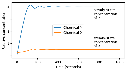
For the parameter values \(k_1=0.1\), \(k_2=0.4\), \(k_3=0.1\) and \(k_4=0.2\), the system results in decaying oscillations of the concentrations \(X\) and \(Y\). Over time the system reaches equilibrium and the values of \(X\) and \(Y\) reach a steady state.

1. Assuming the initial concentrations are zero, run the simulation with the parameters above for \(1000\) time steps. Plot \(X\) and \(Y\) on the same figure.

2. Assuming that the system has reached a steady state after 1000 timesteps, we can define the steady-state concentrations to be \(X_{1000}\) and \(Y_{1000}\). Determine the steady-state values of \(X\) and \(Y\).

3. Write a function steady_state_X(k1, k2, k3, k4) which runs the simulation for the given values of \(k_1\), \(k_2\), \(k_3\) and \(k_4\), then returns the steady-state value of \(X\). Check that it gives the expected value for \(k_1=0.1\), \(k_2=0.4\), \(k_3=0.1\) and \(k_4=0.2\).

ss_x = steady_state_X(0.1, 0.4, 0.1, 0.2)
print(ss_x) # should print the expected value

4. Determine the steady-state val ue of X for \(k_1=0.1\), \(k_2=0.4\), \(k_3=0.1\) and a range of values of \(k_4\) between \(0\) and \(0.3\). Plot the results on a graph with \(k_4\) on the x-axis and the steady-state value of \(X\) on the y-axis.

5. Write a function max_X(k1, k2, k3, k4) which returns the peak value of the concentration of X, then (on the same graph as the previous question) plot the peak concentration of X for \(k_4\) between \(0\) and \(0.3\). (Use the numpy function np.max which returns the maximum value of an array).