Homework solutions
Contents
2.4.2. Homework solutions#
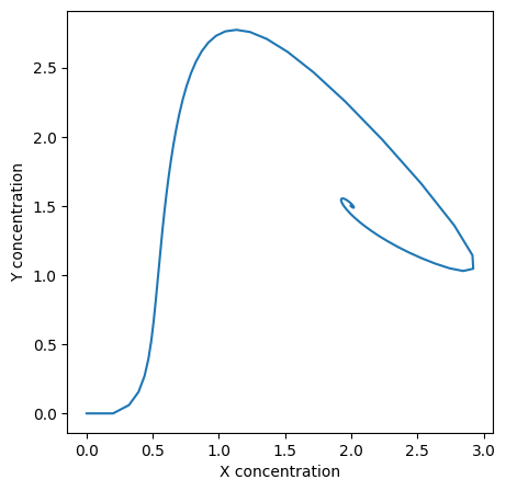
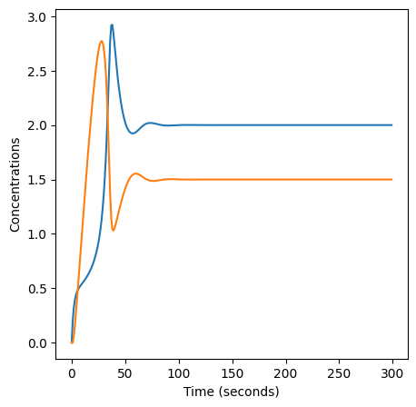
The BZ reaction can be modelled by the following equations, where \(X_i\) and \(Y_i\) are the concentrations of the two reactants X (red) and Y (colourless) at timestep \(i\). At each timestep, the concentrations of the two reactants change according to the difference equations below. Each timestep has a duration of one second.
Model the evolution of the chemical reaction for \(300\) seconds, assuming the initial concentrations are zero, and using the parameter values \(k_1=0.2,k_2 = 0.4, k_3 = 0.1\mathrm{~and~}k_4 = 0.3\).
Experiment with different values of \(k_1\). For what range of values of \(k_1\) does the reaction exhibit oscillations?
2.4.2.1. Modelling#
First, to model the equations we can follow the same structure we used in the tutorial. To see how the reactants interact we can model both concentrations on the same graph.
# import necessary libraries
import numpy as np
import matplotlib.pyplot as plt

# set up variables and arrays
n = 300
k1 = 0.2
k2 = 0.4
k3 = 0.1
k4 = 0.3

X = np.zeros(n)
Y = np.zeros(n)

# initialise variables (not strictly necessary here!)
X[0] = 0
Y[0] = 0

# implement equations
for i in range(n - 1):
    X[i+1] = X[i] + k1 - k2*X[i] + k3*(X[i]**2)*Y[i]
    Y[i+1] = Y[i] + k4*X[i] - k3*(X[i]**2)*Y[i]

# plot so we can see what happens
plt.figure(figsize=(5,5))
plt.plot(X, Y)
plt.xlabel("X concentration")
plt.ylabel("Y concentration")

plt.figure(figsize=(5,5))
plt.plot(X)
plt.plot(Y)
plt.xlabel("Time (seconds)")
plt.ylabel("Concentrations")
Text(0, 0.5, 'Concentrations')
2.4.2.2. Experiment with \(k_1\)#
We can use np.linspace to test a few different values for \(k_1\). Let’s try the interval \([0, 0.3]\).
for k1 in np.linspace(0, 0.3, 20):

    X = np.zeros(n)
    X[0] = 0
    Y = np.zeros(n)
    Y[0] = 0

    for i in range(n - 1):
        X[i+1] = X[i] + k1 - k2*X[i] + k3*X[i]**2*Y[i]
        Y[i+1] = Y[i] + k4*X[i] - k3*X[i]**2*Y[i]

    plt.figure(figsize=(5,5))
    plt.plot(X, Y)
    plt.xlabel("X concentration")
    plt.ylabel("Y concentration")
    plt.title(k1) # add title to each figure so we can see what the value is

    plt.figure(figsize=(5,5))
    plt.plot(X)
    plt.plot(Y)
    plt.xlabel("Time (seconds)")
    plt.ylabel("Concentrations")
    plt.title(k1) # add title to each figure so we can see what the value is
c:\users\natsciteaching\appdata\local\programs\python\python37\lib\site-packages\ipykernel_launcher.py:9: RuntimeWarning: overflow encountered in double_scalars
  if __name__ == "__main__":
c:\users\natsciteaching\appdata\local\programs\python\python37\lib\site-packages\ipykernel_launcher.py:10: RuntimeWarning: overflow encountered in double_scalars
  # Remove the CWD from sys.path while we load stuff.
c:\users\natsciteaching\appdata\local\programs\python\python37\lib\site-packages\ipykernel_launcher.py:9: RuntimeWarning: invalid value encountered in double_scalars
  if __name__ == "__main__":
c:\users\natsciteaching\appdata\local\programs\python\python37\lib\site-packages\ipykernel_launcher.py:10: RuntimeWarning: invalid value encountered in double_scalars
  # Remove the CWD from sys.path while we load stuff.
c:\users\natsciteaching\appdata\local\programs\python\python37\lib\site-packages\ipykernel_launcher.py:12: RuntimeWarning: More than 20 figures have been opened. Figures created through the pyplot interface (`matplotlib.pyplot.figure`) are retained until explicitly closed and may consume too much memory. (To control this warning, see the rcParam `figure.max_open_warning`).
  if sys.path[0] == "":
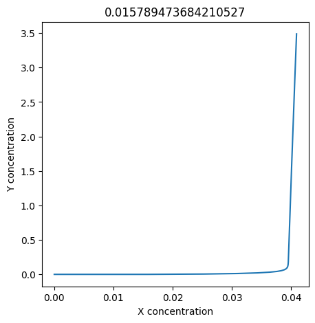
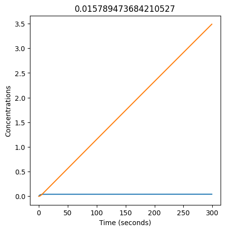
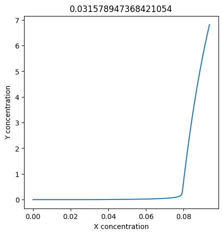
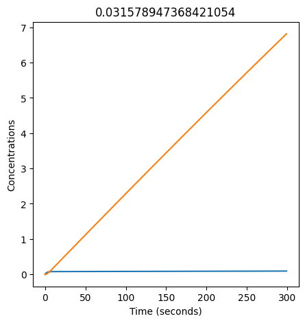
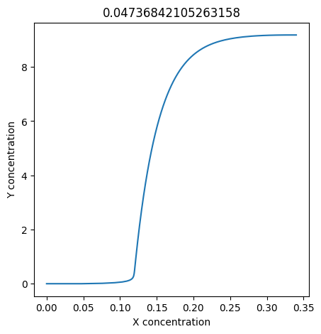
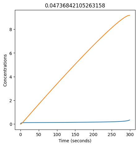
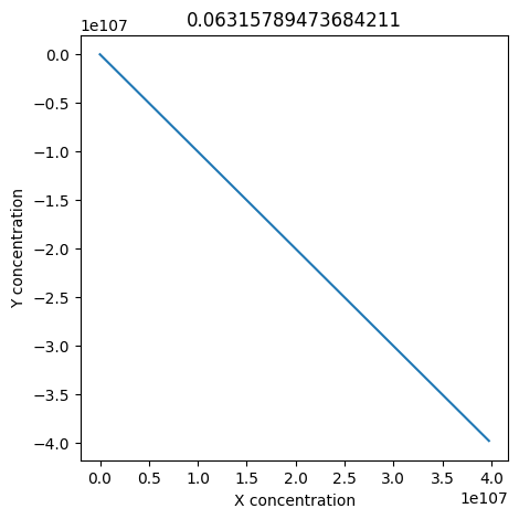
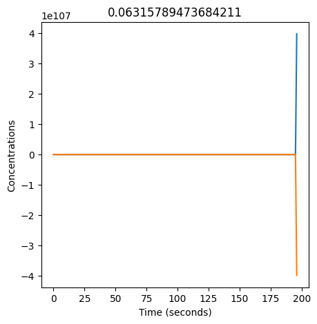
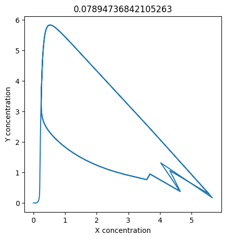
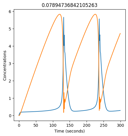
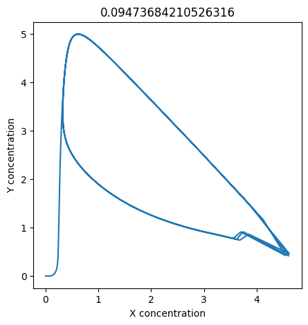
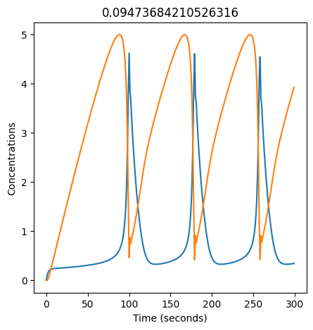
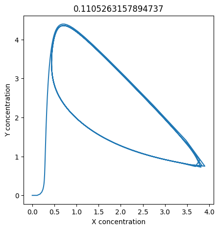
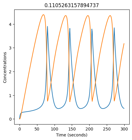
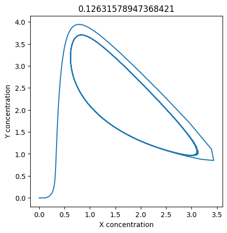
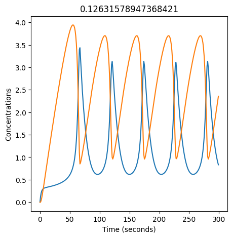
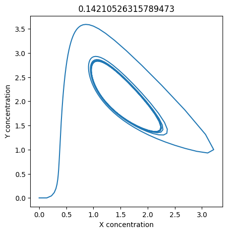
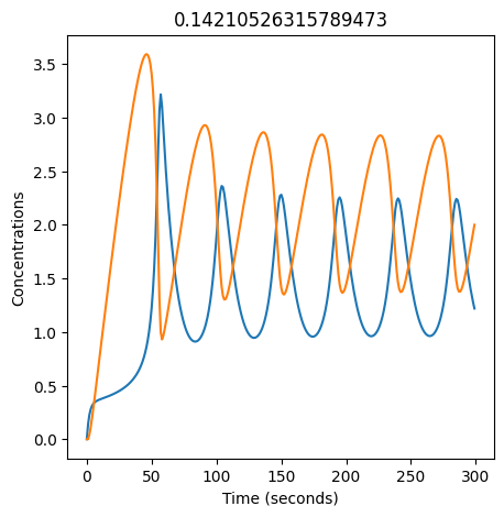
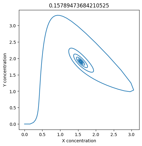
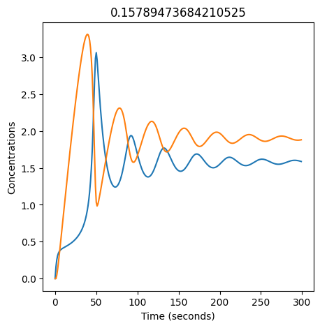
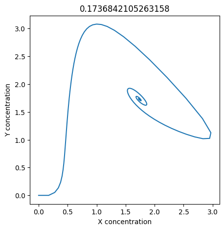
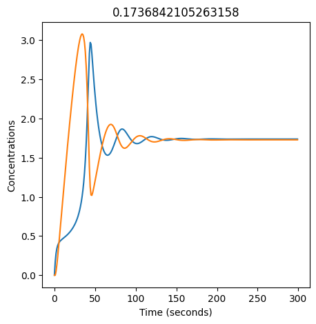
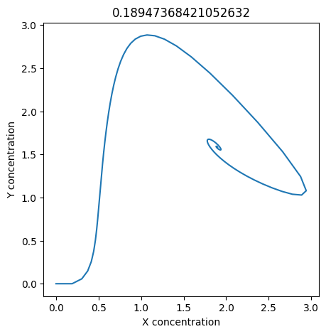
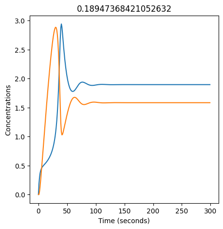
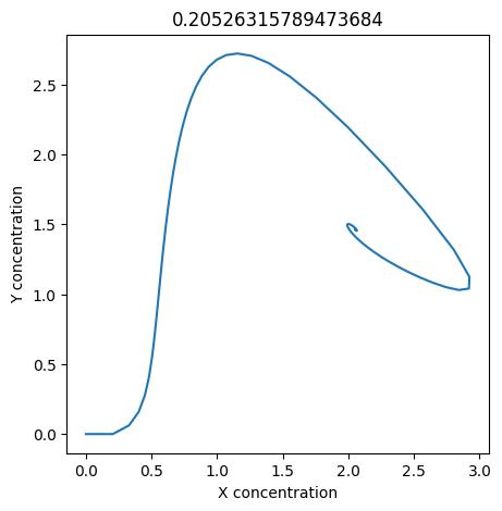
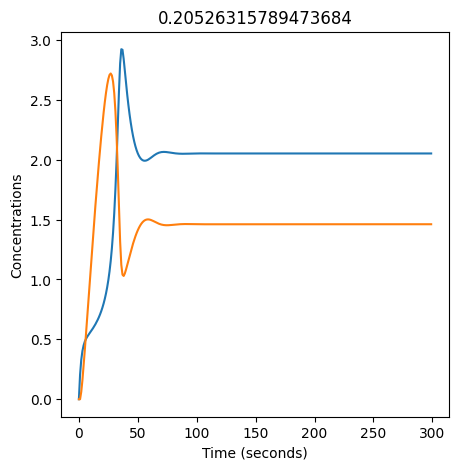
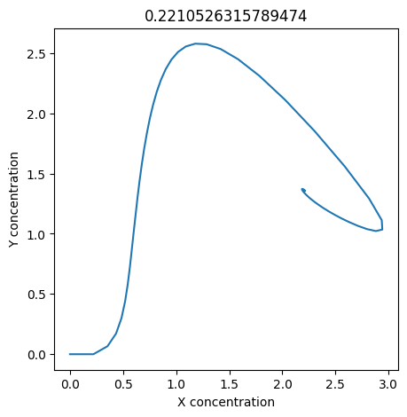
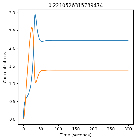
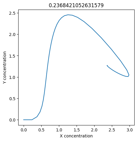
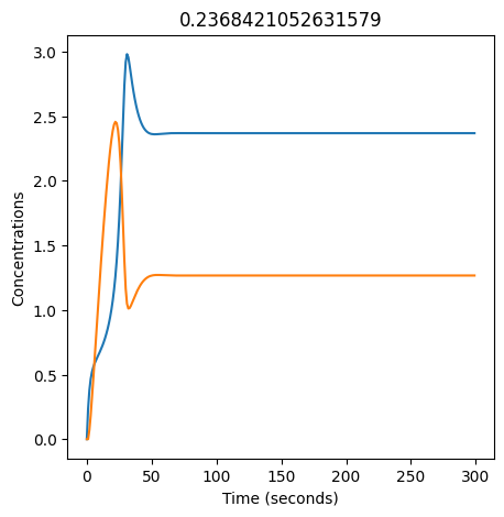
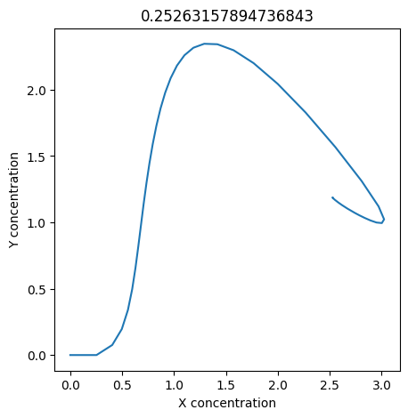
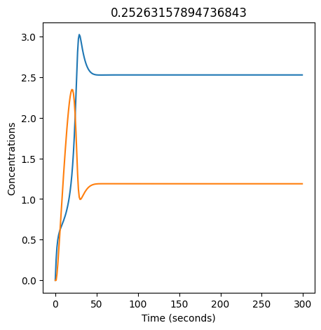
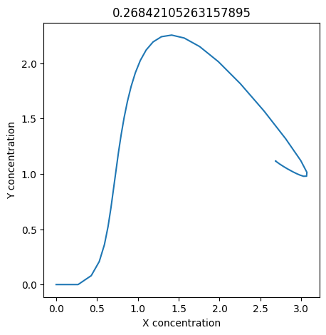
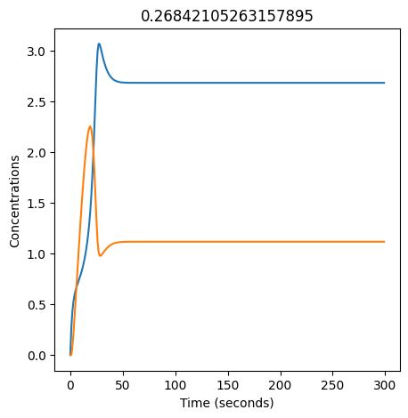
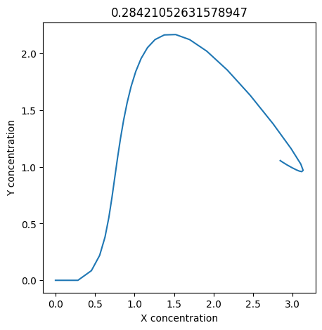
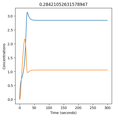
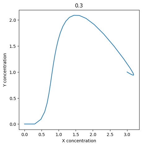
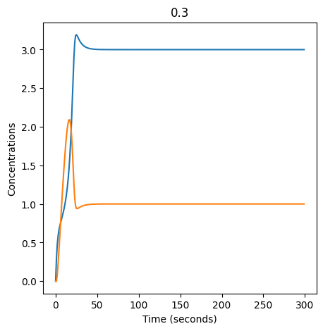
We see oscillations first appear when \(k_1 \approx 0.079\), these continue until \(k_1 \approx 0.25\) when \(X\) stops oscillating.

