1. Introduction to Graphs

Attention

All exercises in Section 1 should be completed using pen and paper. We won’t be touching a computer keyboard until Section 2.

A graph is a collection of nodes (or vertices) connected by edges. In the following example, which represents part of the egg-laying circuit of C-Elegans, nodes represent neurons and edges represent synaptic connections between them:

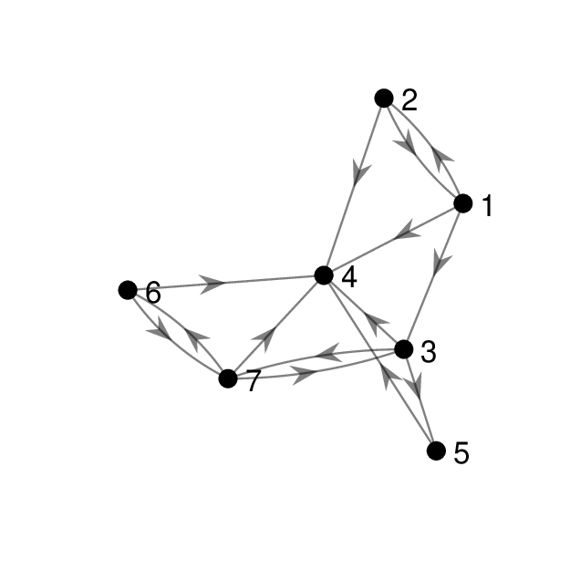
Fig. 1.1 Directed graph of the egg-laying circuit of C-Elegans.

Definitions

Graph

A graph \(G = (V, E)\) is a set of nodes \(V = \{v_1, v_2, \dots, v_n\}\) and edges \(E = \{(v_i, v_j), \dots\}\) where \((v_i, v_j)\) is an edge joining nodes \(v_i\) and \(v_j\).

Order

The order of a graph \(G\) is number of nodes in \(G\).

Directed Graph

A directed graph (or digraph) is a graph where each edge \((v_i, v_j)\) has an associated direction from \(v_i\) to \(v_j\).

Simple Graph

A simple graph is a graph which does not have any loops (edges from a node to itself) or multiple edges (two edges joining the same two nodes in the same direction).

Multigraph

A multigraph is a graph which is not a simple graph.

In this course we will mostly be considering simple directed graphs, since these are the most useful for representing neural circuits.

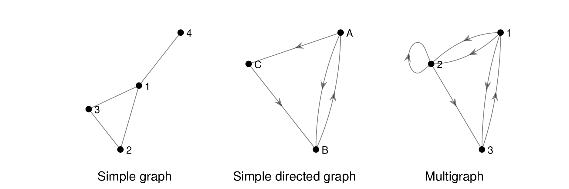
Fig. 1.2 Simple, directed and multigraphs.

1.1. Graph Representations

Given a graph, we would like to be able to answer various questions: Do two graphs have the same structure? Is there a path from node X to node Y? What is the minimum length path from node X to node Y? To answer these questions, we need a way to represent the graph computationally. There are three main ways to represent a graph: edge list, adjacency list and adjacency matrix.

Definitions

Edge List

An edge list consists of a list of pairs of numbers, one pair for each edge. The numbers represent the starting and ending nodes of each edge. Here is the edge list corresponding to the egg-laying graph:

\[\begin{split}[1, 2], [1, 3], [1, 4], [2, 1], [2, 4], [3, 4], [3, 5],\\ [3, 7], [5, 4], [6, 4], [6, 7], [7, 3], [7, 4], [7, 6]\end{split}\]

For a directed graph, the order that we write the pair \([i, j]\) is important, but the order that we write the list of pairs is not.

Adjacency List

An adjacency list consists of a sequence of lists. The list at position \(i\) contains all the nodes which node \(i\) connects to. Here is the adjacency list corresponding to the egg-laying graph:

\[[2, 3, 4], [1, 4], [4, 5, 7], [], [4], [4, 7], [3, 4, 6]\]

Adjacency Matrix

An adjacency list consists of a sequence of lists. The list at position \(i\) contains all the nodes which node \(i\) connects to. Here is the adjacency list corresponding to the egg-laying graph:

\[\begin{split} \begin{bmatrix} 0 & 1 & 1 & 1 & 0 & 0 & 0\\ 1 & 0 & 0 & 1 & 0 & 0 & 0\\ 0 & 0 & 0 & 1 & 1 & 0 & 1\\ 0 & 0 & 0 & 0 & 0 & 0 & 0\\ 0 & 0 & 0 & 1 & 0 & 0 & 0\\ 0 & 0 & 0 & 1 & 0 & 0 & 1\\ 0 & 0 & 1 & 1 & 0 & 1 & 0 \end{bmatrix} \end{split}\]

Exercise 1.1

For the following directed graph, write out its:

1. Edge list.

2. Adjacency list.

3. Adjacency matrix.

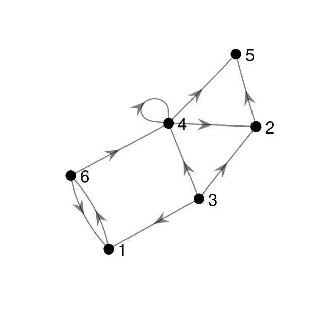
Exercise 1.2

Draw a picture of the directed graph defined by:

1. Edge list \( [1, 2], [5, 4], [5, 5], [5, 3], [3, 1], [1, 3], [3, 4], [4, 1]\)

2. Adjacency list \([2, 3], [], [1, 4], [1], [5, 4, 3]\)

3. Adjacency matrix:

\[\begin{split} \begin{bmatrix} 0 & 0 & 0 & 0 & 1 & 0\\ 0 & 0 & 0 & 0 & 0 & 0\\ 1 & 0 & 0 & 1 & 0 & 0\\ 0 & 1 & 0 & 0 & 0 & 1\\ 0 & 0 & 0 & 0 & 0 & 1\\ 0 & 0 & 0 & 1 & 0 & 0 \end{bmatrix} \end{split}\]

Two of the three graphs are the same. Which two?

1.2. Walks and Paths

A walk in a graph is a sequence of nodes formed by following edges. A walk may visit the same node several times. For example, in the egg-laying graph \([1, 3, 7, 6]\) is a walk from node 1 to node 6, and \([1,2,1,3]\) is a walk from node 1 to node 3.

A path is a walk which does not visit any node more than once. So \([1, 3, 7, 6]\) is a path but \([1, 2, 1, 3]\) is not.

The length of a walk (or path) is the number of edges (which is one less than the number of nodes).

Exercise 1.3

1. The complete directed graph \(K_n\) is a directed graph with \(n\) nodes and an edge connecting every node to every other node (but no node is connected to itself). Sketch \(K_3\). In \(K_3\), how many distinct length 10 walks are there?

2. In the egg-laying circuit, identify all paths from node 6 to node 4, and all paths from node 4 to node 6.

3. Find the longest path in the egg-laying circuit.

1.3. Shortest Paths

Given two nodes in a directed graph, there may be zero, one or multiple paths between them. The path distance from node \(v_i\) to node \(v_j\) is the length of the shortest path connecting \(v_i\) to \(v_j\). In this section we will build an algorithm which calculates the path distance between nodes, using a technique called breadth first search.

Exercise 1.4

Determine the path distance between node 1 and every other vertex in the egg-laying circuit by completing the following steps:

1. Label node 1 with a distance of 0.

2. Label every node directly connected by an edge from node 1 with a distance 1.

3. Label every unlabelled node directly connected by an edge from a distance-1 node with a distance of 2.

4. Continue until the whole graph is labelled.

1.4. Breadth First Search

Exercise 1.4 should have given you an intuition about how to build an algorithm which calculates the shortest path between the starting node and every other node. In the next section we explore this technique.

A search algorithm is a method of traversing a graph by following edges. In breadth first search (BFS), we start at the origin node and traverse the graph in levels, increasing the distance from the origin one level at a time.

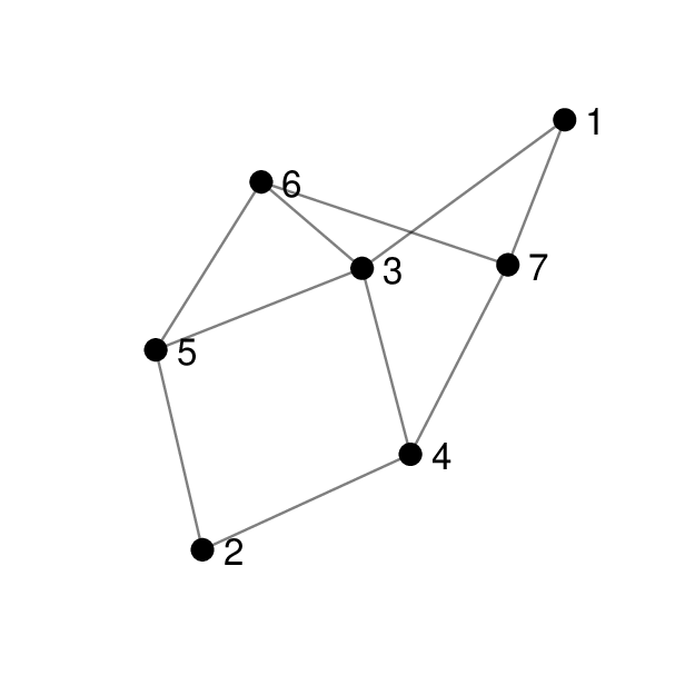
Example

Compute a breadth first search of the undirected graph above, starting from node 1.

At the first level, we visit the direct neighbours of node 1, which are nodes 3 and 7. In the second level, we visit nodes 4, 5 and 6 which are the direct neighbours of nodes 3 and 7. Finally, we visit node 2 which is the direct neighbour of nodes 4, 5 and 6. The output of the breadth first search is \([1, 3, 7, 4, 5, 6, 2]\).

Note that within each level, the nodes may be visited in any order.

Exercise 1.5

1. Compute a breadth first search of the egg-laying graph, starting from node 2, and use this to determine the path distance of each node from node 2.

2. Do the same starting from node 6.

1.5. Connectedness

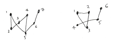
An undirected graph is connected if there is a path between every node and every other node. Otherwise, we say that the graph is disconnected.

If a graph is not connected, then we can split it into connected components by declaring that two vertices are in the same component if and only if there is a path between them.

In the example below, the left hand graph is connected. The graph on the right is disconnected with two components \([1, 2, 3]\) and \([4, 5, 6]\).

Exercise 1.6

Use breadth first search to determine all connected components of the undirected graph given by the edge list \([1, 7], [2, 3], [6, 9], [5, 7], [8, 4], [10, 2], [5, 6], [5, 1]\).

1. Draw the graph.

2. Choose any node as the starting point of BFS. All nodes visited by the BFS belong to a single component.

3. Choose any unvisited node as the starting point of a new BFS.

4. Continue until all nodes have been allocated to a component.

1.6. References

[1] Sporns, Olaf. Graph theory methods for the analysis of neural connectivity patterns. In Neuroscience Databases. Springer, Boston, MA, 2003. pp 171-185.

[2] Fornito, A., Zalesky, A., and Bullmore, E. Fundamentals of Brain Network Analysis. Academic Press, 2016.