15. Electrostatics

15.1. Coulombs Law

Lets start with the basics, Coulombs law in Equation (15.1), tells us that a repulsive force between two charges $Q_i$, $Q_1$ at the origin and $Q_2$ at distance $r$:

(15.1)$$F_c=\frac{Q_1{Q}_2}{4\pi {ϵ}_0}\frac{1}{r^2}$$

Obviously we can shift the charges, so that in general $(Q_1({\mathbf{r}}_1),Q_2({\mathbf{r}}_2))$. Also ${\mathbf{F}}_c$ is a vector quantity, so we can write the force acting on $Q_2({\mathbf{r}}_2)$ due to $Q_1({\mathbf{r}}_1)$ as:

$${\mathbf{F}}_{12}=\frac{Q_1{Q}_2}{4\pi {ϵ}_0}\frac{1}{|{\mathbf{r}}_1-{\mathbf{r}}_2{|}^2}{\hat{\mathbf{r}}}_{12}$$

where ${\hat{\mathbf{r}}}_{12}$ is a normalised vector that points from $Q_1({\mathbf{r}}_1)\to Q_2({\mathbf{r}}_2)$. This force is related directly to the size of the charges and to the inverse square of the distance between them. We can define the Electric Field as the force per unit charge, in this case we can find the electric field due to the charge $Q_1$ measured at ${\mathbf{r}}_2$ as:

(15.2)$$\mathbf{E}=\frac{{\mathbf{F}}_c}{Q_2}=\frac{Q_1}{4\pi {ϵ}_0}\frac{1}{|{\mathbf{r}}_1-{\mathbf{r}}_2{|}^2}{\hat{\mathbf{r}}}_{12}$$

This expression has $Q_1$ taking the role of a Source Charge. If we have a point charge, we can draw the electric field around it, as shown in Fig. 15.1.

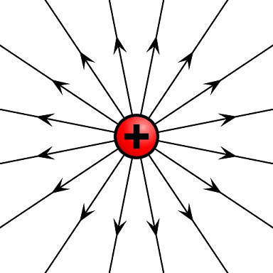
Fig. 15.1 Electric fields lines from a positive charge

Our field lines radiate outwards radially, depending only on the distance from a point to the charge (here we are just assuming a point charge) and in the direction a positive charge would follow (here outwards as like charges repel).

These are all very sound ideas that we have no doubt learnt before, the question is whilst Coulombs law is a very effective tool to empirically describe electric fields from point charges, where does is arrive from? Will it work in more complicated situations?

15.2. Superposition of charges

15.3. Infinitesimal Coulombs law

Lets start with a simpler problem first though, a semicircular arc of charge, as depicted in Fig. 16.9

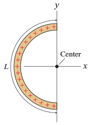
Fig. 15.2 An finite line of charges, with charge density $\lambda$, arranged in a semicircular arc of length $L$ and centered on the origin.

What are the symmetries of this semicircular system? Well if we consider a section of the arc, it will carry a charge $\mathrm{d}Q$ which we can rewrite as $\mathrm{d}Q=\lambda \mathrm{d}\ell$. Given that for a circular arc $\ell =r\theta$ and since $L=\pi r$, therefore

$$\mathrm{d}Q=\frac{\lambda L}{\pi }\mathrm{d}\theta$$

where $\theta$ is an angle that moves round the arc, as we define in Fig. 16.10.

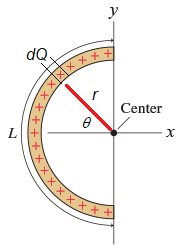
Fig. 15.3 Semicircular arc of charges, centered on the origin, with charge element $\mathrm{d}Q$, length $L$, radius $r$ and angle $\theta$.

Clearly now we want to integrate over all the charges $\mathrm{d}Q$ which will involve integrating over all angles $\mathrm{d}\theta$. Since we are treating these infitesimal charge elements as point charges, the magnitude of the electric field has the form:

$$\mathrm{d}E=\frac{\mathrm{d}Q}{4\pi {ϵ}_0{r}^2}=\frac{\pi \mathrm{d}Q}{4{ϵ}_0{L}^2}$$

The direction of the field components however will change depending on whereabouts along the ring we are, clearly are $\theta =0$, the field is directed along the $x$-axis only:

$$\mathrm{d}{\mathbf{E}}_{\theta =0}=\frac{\pi \mathrm{d}Q}{4{ϵ}_0{L}^2}\hat{\mathbf{i}}+0\hat{\mathbf{j}}$$

Whilst if we examine the field at $\theta =-\pi /2$ and $\theta =\pi /2$, we notice that the electric field will be aligned in the positive and negative $y$-axis directions (respectively):

$$\begin{array}{rlr}\mathrm{d}{\mathbf{E}}_{\theta =-\pi /2}& =& 0\hat{\mathbf{i}}+\frac{\pi \mathrm{d}Q}{4{ϵ}_0{L}^2}\hat{\mathbf{j}}\\ \mathrm{d}{\mathbf{E}}_{\theta =\pi /2}& =& 0\hat{\mathbf{i}}-\frac{\pi \mathrm{d}Q}{4{ϵ}_0{L}^2}\hat{\mathbf{j}}\end{array}$$

In fact we see that there will always be a cancellation of the $y$ components of the electric field from the arc, we can always pair up the components over $-\pi /2\le \theta \le \pi /2$, this leaves just the $x$ components:

$$\begin{array}{rlr}\mathrm{d}{\mathbf{E}}_{\theta }& =& \frac{\pi \mathrm{d}Q}{4{ϵ}_0{L}^2}[\cos (\theta )\hat{\mathbf{i}}+\sin (\theta )\hat{\mathbf{j}}]\\ {\int }_0^{\mathbf{E}}\mathrm{d}{\mathbf{E}}_{\theta }& =& \frac{\pi }{4{ϵ}_0{L}^2}\frac{\lambda L}{\pi }{\int }_{-\pi /2}^{\pi /2}(\cos (\theta )\hat{\mathbf{i}}+\sin (\theta )\hat{\mathbf{j}})\mathrm{d}\theta \\ \mathbf{E}& =& \frac{\lambda }{4{ϵ}_{0}L}[\sin (\theta )\hat{\mathbf{i}}-\cos (\theta )\hat{\mathbf{j}}{]}_{-\pi /2}^{\pi /2}=\frac{\lambda }{2{ϵ}_{0}L}\hat{\mathbf{i}}+0\hat{\mathbf{j}}\end{array}$$

15.3.1. Rectilinear Rod

Lets return to the rod in Fig. 16.8, we can set this system up in Fig. 16.11, trying to make the rod as symmetric as possible:

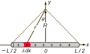
Fig. 15.4 An finite line of charges, with charge density $\lambda$, with length $L$, symmetrically aligned over the $x$ axis. We pick out an element of charge indicated in red, so here $\mathrm{d}Q=\lambda \mathrm{d}x$.

With a line of charge, of length $L$, aligned along the $x$ axis, we can look at a point at a distance $R$ away, aligned halfway along the rod. Once again we can break up this line of charge into infinitesimal chunks, each contributing $\mathrm{d}Q$ charge and then the overall electric field will be found by superposition. The magnitude of the electric field at a distance $R$ from the rod appears to be given by:

$$\mathrm{d}E=\frac{\mathrm{d}Q}{4\pi {ϵ}_0{r}^2}$$

where the length $r$ can take values between $R\le r\le \sqrt{R^2+L^2/4}$.

In this system, we find that at $x=0$, the electric field is only aligned in the $y$ direction:

$$\mathrm{d}{\mathbf{E}}_{x=L/2}=0\hat{\mathbf{i}}+\frac{\mathrm{d}Q}{4\pi {ϵ}_0{R}^2}\hat{\mathbf{j}}$$

whereas the $x$ components of the electric field for all the lengths at $-L/2\le x<0$ and $0>x\le L/2$ will pair up, to cancel out, leaving only the $y$ components:

$$\begin{array}{rlr}\mathrm{d}\mathbf{E}& =& \frac{\mathrm{d}Q}{4\pi {ϵ}_0{r}^2}(\sin (\theta )\hat{\mathbf{i}}+\cos (\theta )\hat{\mathbf{j}})\\ {\int }_0^{\mathbf{E}}\mathrm{d}{\mathbf{E}}^{\prime }& =& \frac{\lambda }{4\pi {ϵ}_0}{\int }_{-L/2}^{L/2}(\frac{x}{r^3}\hat{\mathbf{i}}+\frac{R}{r^3}\hat{\mathbf{j}})\mathrm{d}x\\ \mathbf{E}& =& \frac{\lambda }{4\pi {ϵ}_0}{\int }_{-L/2}^{L/2}(\frac{x}{(x^2+R^2{)}^{3/2}}\hat{\mathbf{i}}+\frac{R}{(x^2+R^2{)}^{3/2}}\hat{\mathbf{j}})\mathrm{d}x\end{array}$$

Where we have used the substitutions $\sin (\theta )=x/r=x/\sqrt{x^2+R^2},\cos (\theta )=R/r=R/\sqrt{x^2+R^2}$. We can also use the substitution $x=R\tan (\theta )\Rightarrow \mathrm{d}x=R{\sec }^2(\theta )$ to find:

$$\begin{array}{rlr}\mathbf{E}& =& \frac{\lambda }{4\pi {ϵ}_0}{\int }_{x=-L/2}^{x=L/2}(\frac{R\tan (\theta )}{R^3{\sec }^3(\theta )}\hat{\mathbf{i}}+\frac{R}{R^3{\sec }^3(\theta )}\hat{\mathbf{j}})R{\sec }^2(\theta )\mathrm{d}\theta \\ & =& \frac{\lambda }{4\pi {ϵ}_{0}R}{\int }_{x=-L/2}^{x=L/2}(\sin (\theta )\hat{\mathbf{i}}+\cos (\theta )\hat{\mathbf{j}})\mathrm{d}\theta \\ & =& \frac{\lambda }{4\pi {ϵ}_{0}R}[-\cos (\theta )\hat{\mathbf{i}}+\sin (\theta )\hat{\mathbf{j}}{]}_{x=-L/2}^{x=L/2}\\ & =& \frac{\lambda }{4\pi {ϵ}_{0}R}[-\frac{R}{(x^2+R^2{)}^{1/2}}\hat{\mathbf{i}}+\frac{x}{(x^2+R^2{)}^{1/2}}\hat{\mathbf{j}}{]}_{-L/2}^{L/2}\\ & =& \frac{\lambda }{4\pi {ϵ}_{0}R}(0\hat{\mathbf{i}}+\frac{L}{(L^2/4+R^2{)}^{1/2}}\hat{\mathbf{j}})\end{array}$$

Which results in:

$$\mathbf{E}=\frac{\lambda L}{4\pi {ϵ}_{0}R\sqrt{L^2/4+R^2}}\hat{\mathbf{j}}$$

Notice that in the limit of $L\gg 1$, this would look like:

$$\mathbf{E}\to \frac{\lambda }{2\pi {ϵ}_{0}R}\hat{\mathbf{j}}$$

which is essentially the result for the infinite line of charge in Equation (16.1).

We note therefore that the relevant expression for the magnitude of the electric field at a distance $R$ from the rod is found from just the $y$ component:

(15.3)$$\begin{array}{rlr}\mathrm{d}E& =& \frac{\mathrm{d}Q}{4\pi {ϵ}_0{r}^2}\cos (\theta )=\frac{\mathrm{d}QR}{4\pi {ϵ}_0{r}^3}\\ \Rightarrow E& =& \frac{\lambda }{4\pi {ϵ}_0}{\int }_{rod}\frac{R}{r^3}\mathrm{d}x=\frac{\lambda }{4\pi {ϵ}_{0}R}[\frac{x}{\sqrt{x^2+R^2}}{]}_{rod}\end{array}$$

15.4. Gauss’s law

Lets now look at electric fields from the point of view of an a containing surface and flux crossing the surface boundary. Starting with a charge $Q$, we can surround this in three dimensions by a sphere, as seen in Figure Fig. 15.5.

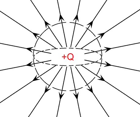
Fig. 15.5 Flux of the electric field from a point charge $+q$ passing through a spherical surface.

Now we have field lines perpendicular to the surface, here a sphere, so a similar situation to hose pipe and the water. But now we have to think about how close the field lines get over the spheres surface - they should really be thought of as infinitesimally small, so we use an area integral summing up the flux crossing the bounding surface area $A$:

$${\mathrm{\Phi }}_E={\iint }_A\mathbf{E}\cdot \mathrm{d}\mathbf{A}$$

What will this flux we related to? Well imagine us increasing the size of the charge at the centre of the sphere, clearly the size of the Coulombic force between this and another charge will increase and so the magnitude of the electric field will increase. As the flux is counting however much of the electric field is crossing the spherical boundary here, clearly the flux will increased, so we can make the statement:

$$\iint \mathbf{E}\cdot \mathrm{d}\mathbf{A}\propto Q$$

This makes sense because both flux and charge are scalar quantities and because the flux only seems to change with the charge linearly (we saw this in Equation (15.2)). Lets just assign a constant $k$ to make this an equation

$$\iint \mathbf{E}\cdot \mathrm{d}\mathbf{A}=kQ$$

and we will aim to find the value of $k$ later. One thing we can find straightforwardly is what units $k$ should have

$$[\text{k}]=[\rho ][\mathbf{v}][\text{Q}{]}^{-2}=\text{kg}{\text{m}}^{-3}\text{m}{\text{s}}^{-1}{\text{C}}^{-2}=\text{kg}{\text{m}}^{-2}{\text{s}}^{-1}{\text{C}}^{-2}$$

We can aim to use this flux law to get to Coulombs law, as the two results must agree, so starting with the spherical surface area $A$ around the charge $Q$ we find that the area normal vector is $\mathbf{A}=A_r\hat{\mathbf{r}}$. The surface integral term therefore reduces to:

$$\iint \mathbf{E}\cdot \mathrm{d}\mathbf{A}=\iint E_r\mathrm{d}{A}_r$$

where we decomposed the electric field $\mathbf{E}$ in to components:

$$\mathbf{E}=E_r\hat{\mathbf{r}}+E_{\theta }\hat{\theta }+E_{\varphi }\hat{\varphi }$$

By symmetry therefore the electric field does not have an angular $(\theta ,\varphi )$ dependence - this makes sense physically because whether a charge is on our left or right hand side does not charge the force felt if it is at the same fixed distance.

Calculating $\iint \mathbf{E}\cdot \mathrm{d}\mathbf{A}$ is straightforward on a sphere:

$$\iint E_r\mathrm{d}{A}_r=\iint E_r{r}^2\sin \theta \mathrm{d}\theta \mathrm{d}\varphi$$

Since $E_r$ only has $r$ dependence, we can factorise this out of the integral:

$$\begin{array}{rlr}{E}_r\iint r^2\sin \theta \mathrm{d}\theta \mathrm{d}\varphi =E_r(4\pi r^2)& =& kQ\\ \Rightarrow E_r& =& \frac{kQ}{4\pi r^2}\end{array}$$

Finally we can write this in vector form:

$$\mathbf{E}=E_r\hat{\mathbf{r}}=\frac{kQ}{4\pi r^2}\hat{\mathbf{r}}$$

Comparing this result with Coulomb’s law in Equation (15.1), we find we can fix $k=1/{ϵ}_0$ (which also has the required units, check this for yourself!). So our final expression, which is known as Gauss’s Law, can be written as:

(15.4)$${\iint }_A\mathbf{E}\cdot \mathrm{d}\mathbf{A}=\frac{Q}{{ϵ}_0}$$

The charge $Q$ here should be carefully explained, central to the discussion of the flux were the field lines from the charge cutting the bounding surface area $A$, so we really mean to write the $Q$ as one enclosed by the area $A$ and so we should really write Gauss’s law as:

$${\iint }_A\mathbf{E}\cdot \mathrm{d}\mathbf{A}=\frac{Q_{enclosed}}{{ϵ}_0}$$

15.5. Gravitational Analogue

One of the grand goals of physics is to understand nature through the same equations but on different scales - so called universality. We find that the equations in electrostatics can be used to discuss Newton’s law of gravitation. We notice that the equations are essentially just a redefinition of fields and constants:

$$F_C=\frac{1}{4\pi {ϵ}_0}\frac{Q_1{Q}_2}{r^2}⟺F_G=-G\frac{M_1{M}_2}{r^2}$$

where $F_G$ is negative as it is only an attractive force, these suggest that by analogy:

$$\frac{1}{{ϵ}_0}⟺-4\pi G,Q_i⟺M_i$$

Our electric field here $\mathbf{E}$ has a direct analogue in the gravitational field $\mathbf{g}$:

$$\mathbf{E}=\frac{{\mathbf{F}}_E}{Q}⟺\mathbf{g}=\frac{{\mathbf{F}}_N}{M}$$

and therefore we could examine Gauss’s law for gravitational fields:

(15.5)$$\iint \mathbf{g}\cdot \mathrm{d}\mathbf{A}=-4\pi G{M}_{enclosed}$$

An application of this is understanding the interior gravitational field of a large uniform astrophysical body (e.g. the Earth), which we find results in the analogue of Fig. 16.3.