3. Harmonic and Oscillatory Motion

Waves are connected to oscillations and describe the transfer of energy from different parts of a system through oscillating phenomena within said system. This should be seen differently to other ways that energy may be transferred, e.g. thermodynamically or by doing work by applying a force over a distance. The study of oscillations can be started by looking at the simplest kind of oscillating system, that of Simple Harmonic Motion (SHM) and Simple Harmonic Oscillators (SHO), before moving on to consider damped and forced harmonic systems.

3.1. Simple Harmonic Motion

Lets consider a simple system with a mass on a idealised spring, which follows Hooke’s law

\[\bf{F}_H = k \bf{x}\]

where \(\bf{F}\) is the force applied, \(x\) is the extension measured in the spring from the application of the force \(\bf{F}\) and \(k\) is the spring constant, a material property of the spring.

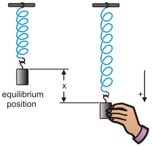
Fig. 3.1 Mass on a spring demonstrating SHM

As we see in Fig. 3.1, a mass hanging from a spring will settle into an equilibrium position where the downward weight from the mass \(\bf{W}\) (the spring here is considered mass-less) and the upward tension \(\bf{F}_H\) from the spring balance out, producing no net force and therefore no net acceleration (by Newton’s second law). At this equilibrium position the spring extension will be denoted by \(\bf{e}\):

\[\Sigma \bf{F} = m\bf{a} \Rightarrow \bf{W} - k\bf{e}\]

If we displace the mass downwards, with an additional extension \(\bf{x}\) (which we have denoted is the positive direction), then the Hooke’s law tension from the spring will be directed upwards (which will be in the negative direction)

\[\Sigma \bf{F} = m\bf{a} \Rightarrow \bf{W} - k(\bf{e} + \bf{x}) = m\bf{a}\]

we can express the acceleration \(\bf{a}\) in terms of a second derivative of the displacement \(\bf{x}\) so we can rewrite as

\[\ddot{\bf{x}}= - \frac{k}{m}\bf{x}\]

which is often rewritten as

\[\ddot{\bf{x}} = -{\omega_0}^2\bf{x}\]

where we denote \(\omega_0 = \sqrt{k/m}\) is the natural angular frequency of this system.

Recall from our discussions of calculus that we can solve this second order ODE to give:

(3.1)\[x(t) = A \cos(\omega_0 \,t) + B \sin(\omega_0 \,t) \]

To solve for \(A,\,B\) here we need initial conditions, which we could consider from the physical situation of displacing the mass from equilibrium to an additional displacement \(x = 1\) and then releasing the mass from rest and examining the resulting motion. This tell us that \(x(t = 0) = 1\) and \(\dot{x}(t=0) = v(t = 0) = 0\) and therefore:

\[\begin{split}x(t) &= A \cos(\omega_0 \,t) + B \sin(\omega_0 \,t) \Longrightarrow x(0) = A = 1 \\ \dot{x}(t) &= - \omega_0 A \sin(\omega_0 \,t) + B \omega_0 \cos(\omega_0 \,t) \Longrightarrow \dot{x}(0) = B \omega_0 = 0\end{split}\]

which gives us \(A = 1,\, B = 0\) and so

\[x(t) = \cos(\omega_0\,t)\]

We say this system presents Simple Harmonic Motion (SHM), because it represents the simplest kind of harmonic (also called oscillating or repetitive) motion that we can have. We put energy into the system by extending the spring (which is a form of potential energy \(E_k = \frac{1}{2}kx^2\)) and then this is converted into kinetic energy and then back into potential (this time as gravitational potential energy) as the mass oscillates up and down. What is truly stunning about this system is that SHM can be seen a many different systems but always has the same hallmarks - there is some natural angular frequency \(\omega_0\) we can find from the equations of motion and the energy in the system oscillates between potential and kinetic.

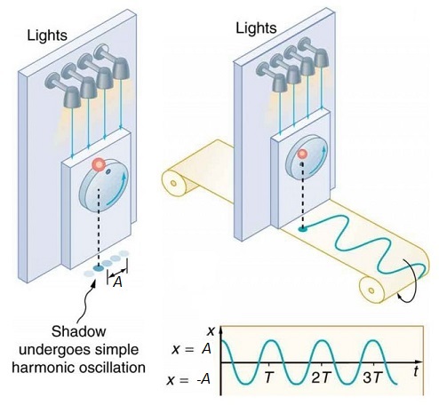
Fig. 3.2 Projection of a ball on a spinning wheel undergoing uniform circular motion, the balls shadow displays SHM - this stretched out in time shows wave motion.

Another feature of this motion is the similarities it brings to circular motion, in fact we can see from Fig. 3.2 that uniform circular motion projected into one dimension is just SHM. The natural angular frequency of the system \(\omega_0\) here is now the angular speed \(\omega\) of the circular motion

\[\omega = \frac{\textrm{d}\theta}{\textrm{d}t}\]

3.2. Energy in a Simple Harmonic System

Going back to the mass and spring system, we can also think about the stored energy in the system,

\[E = KE + PE\]

where the kinetic energy has the usual defintion, \(KE = \frac{1}{2}mv^2 = \frac{1}{2}m{\dot{x}}^2\) and the potential energy is elastic potential energy \(PE = \frac{1}{2}kx^2\), but in a different system this could be replaced with the relevant form of potential. Using the solutions for SHM, (3.1):

\[\begin{split}x(t) &= A \cos(\omega_0 \,t) + B \sin(\omega_0 \,t) \\ \dot{x}(t) &= \omega_0(-A \sin(\omega_0 \,t) + B \cos(\omega_0 \,t) )\\ \Rightarrow E &= \frac{1}{2}m{\omega_0}^2(-A \sin(\omega_0 \,t) + B \cos(\omega_0 \,t) )^2 + \frac{1}{2}k(A \cos(\omega_0 \,t) + B \sin(\omega_0 \,t) )^2\end{split}\]

Given that \({\omega_0}^2 = k / m\), this can be expanded and tidied up becoming:

(3.2)\[E = \frac{1}{2}k\left(A^2 + B^2\right)\]

Which therefore means that the total amount of energy in the system is a constant, even if the energy flucuates between kinetic and potential in the course of the harmonic motion.

3.3. Damped Motion and Forced Harmonic Systems

This SHM model presupposes that there are no losses in energy in this system and this is not always a good model for real world systems, usually there are damping terms in our equations of motion, often this is due to air resistance but can also be caused by frictional forces. This has the effect of adding a first derivative term to the equations of motion

\[m\frac{\mathrm{d}^2 x}{\mathrm{d}t^2} + c \frac{\mathrm{d} x}{\mathrm{d} t} + kx = 0 \]

We could also think of oscillating systems, such as an AC electrical system with an input voltage \(V = V_0 \cos(\Omega t)\), pushing round a current \(I = I_0\cos(\omega t)\) and with some fixed resistances \(R\). Such systems can be described as forced harmonic osciallators, because energy is constantly being put into and given out from the system. The most general form of these systems can be written as:

\[a\frac{\mathrm{d}^2 x}{\mathrm{d}t^2} + b \frac{\mathrm{d} x}{\mathrm{d} t} + cx = F(t)\]

where \(F(t)\) is the driving term. We can rewrite in the :

\[\frac{\mathrm{d}^2 x}{\mathrm{d}t^2} + 2\zeta\omega_0 \frac{\mathrm{d} x}{\mathrm{d} t} + {\omega_0}^2 x = F(t) \]

where \(\omega_0\) is the natural angular frequency of the system and \(\zeta\) is the damping ratio. Often energy is put into the system at a rate of \(\Omega\), e.g. \(F(t) = F_0 \cos(\Omega \,t)\).

3.3.1. Homogeneous (undriven) solutions

This being the case, we can solve this ODE, first with a homogeneous solution using \(x = A_\lambda\,e^{\lambda t}\):

\[\frac{\mathrm{d}^2 x}{\mathrm{d}t^2} + 2\zeta\omega_0 \frac{\mathrm{d} x}{\mathrm{d} t} + {\omega_0}^2 x = A\,e^{\lambda t}\Big( \lambda^2+ 2 \zeta\,\omega_0\,\lambda + {\omega_0}^2 \Big) = 0\]

Solving this resulting quadratic gives:

\[\lambda = \frac{-2\zeta\omega_0 \pm \sqrt{4 \zeta^2{\omega_0}^2-4 {\omega_0}^2}}{2} = \omega_0\Big(-\zeta \pm \sqrt{\zeta^2-1} \Big)\]

This shows that in the homogeneous case, there are three important values of \(\zeta\):

1. Under damping

\(\zeta < 1\), which means the solutions are \(\lambda = \omega_0\Big( -\zeta \pm\ i \sqrt{|1 - \zeta^2|}\Big) = \omega_0\Big(-\zeta \pm i \gamma \Big)\), which is clearly a complex solution and therefore corresponds to oscilating solutions:

\[x(t) = \exp(-\omega_0\,\zeta \,t)\Big(A\cos(\omega_0 \,\gamma t) + B\sin(\omega_0 \,\gamma \,t)\Big)\]

where \(A,\,B\) are constants to be found and \(\gamma^2 = 1- \zeta^2\). We notice that we have factorised the damping term at the start of the expression, this results in damped harmonic oscilations.

2. Critical damping

\(\zeta = 1\), hence \(\lambda = -\omega_0\) which is a repeated root, so the solutions here have the form:

\[x(t) = \exp(- \omega_0\,t)\Big(A + Bt\Big)\]

where \(A,\, B\) are constants to be found. We notice that this is overall a damped solution, no oscillations.

3. Over damping

\(\zeta > 1\), hence \(\lambda = \omega_0\Big(-\zeta \pm \sqrt{\zeta^2-1} \Big) = \omega_0 \Big( -\zeta \pm \delta \Big)\) and so the solutions are of the form:

\[x(t) = A\,\exp(-\omega_0\,(\zeta-\delta)\,t) + B\,\exp(-\omega_0\,(\zeta + \delta)\,t)\]

where \(A,\, B\) are constants to be found and \(\delta^2 = \zeta^2 - 1\). We notice that both of these solutions are decaying, since \(\zeta > \delta\).

We plot examples of all three solutions (using some python code) in figure Fig. 3.3.

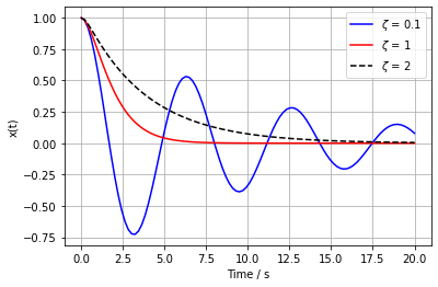
Fig. 3.3 Solutions for the damped harmonic oscillator with \(\zeta = 0.1,\, 1,\, 2\) values.

3.3.2. Inhomogeneous (driven) solutions

Taking into account the driving term, we find that there are additional solutions here:

\[x(t) = x_{h}(t) + x_{d}(t)\]

where \(x_h(t)\) are the homogeneous solutions described in the previous section and \(x_d(t)\) is the (particular integral) contribution from the driving term. For \(F(t) = F_0 \cos(\Omega \,t)\), we find that:

\[\begin{split}x_d(t) &= C\cos(\Omega \,t) + D\sin(\Omega \,t)\\ \frac{\mathrm{d}}{\mathrm{d}t} x_d(t) &= \Omega\Big(-C \sin(\Omega \,t) + D\cos(\Omega \,t) \Big) \\ \frac{\mathrm{d}^2}{\mathrm{d}t^2} x_d(t) &= -\Omega^2 \Big(C\cos(\Omega \,t) + D\sin(\Omega \,t)\Big)\end{split}\]

and therefore we find simultanenous equations arise in \(C,\, D\):

\[\begin{split}\cos(\Omega\,t)\Big[ -C\Omega^2 + 2 D \,\zeta\,\omega_0 + {\omega_0}^2\,C \Big] &= F_0\,\cos(\Omega\,t) \\ \sin(\Omega\,t)\Big[ -D\Omega^2 - 2 C \,\zeta\,\omega_0 + {\omega_0}^2\,D\Big] &= 0 \\ &\,\end{split}\]

This means that:

\[\begin{split}C &= \frac{{\omega_0}^2-\Omega^2}{2\,\zeta\,\omega_0\,\Omega}D \\ C &= \frac{F_0 -2 \zeta\,\omega_0\,\Omega\,D}{{\omega_0}^2 - \Omega^2}\end{split}\]

and therefore:

\[D = \frac{2\zeta\,\omega_0\,\Omega}{({\omega_0}^2 - \Omega^2)^2 + 4\zeta^2\,{\omega_0}^2\,\Omega^2}F_0,\, \quad C = \frac{{\omega_0}^2 - \Omega^2}{({\omega_0}^2 - \Omega^2)^2 + 4\zeta^2\,{\omega_0}^2\,\Omega^2}F_0\]

which means the final solution is found as:

\[x(t) = x_h(t) + \frac{({\omega_0}^2 - \Omega^2)\cos(\Omega\,t) + 2\zeta\,\omega_0\,\Omega\,\sin(\Omega\,t)}{({\omega_0}^2 - \Omega^2)^2 + 4\zeta^2\,{\omega_0}^2\,\Omega^2}\]

If we have some oscillating solutions and find the driven frequency \(\Omega\) coincides with the natural frequency \(\omega_0\), i.e. in the limit of \(\Omega \rightarrow \omega_0\), this gives rise to the phenomena of resonance. We can see this in the solutions:

\[x(t) \simeq \exp(-\Omega\,\zeta \,t)\Big(A\cos(\Omega \,\gamma t) + B\sin(\Omega \,\gamma \,t)\Big) +\frac{\sin(\Omega\,t)}{2\zeta\,\Omega^2}\]

and given that \(0<\zeta <1\) in this case, this second term is enhanced. Resonance can also occur in systems with other types of dampning too and we see the effect of resonance in Fig. 3.4.

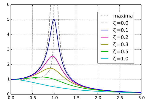
Fig. 3.4 Steady-state variation of amplitude with relative frequency \({\displaystyle \omega /\omega _{0}}\) and damping \({\displaystyle \zeta }\) of a driven harmonic oscillator.