23. Solutions to Maxwell’s Equations

23.1. Electromagnetic Waves

Using Maxwell’s equations, we can see that there are two scalar equations and two vector equations, in the form of coupled ODEs. Lets rewrite these in terms of one field and then try to solve. Recall the Lagrange identity for \(\nabla\) with a vector \({\bf A}\):

\[\nabla \times \left(\nabla \times {\bf A}\right) = \nabla (\nabla \cdot {\bf A}) - \nabla^2 {\bf A} \]

If we take the curl of Equation (22.4):

\[\nabla \times \left(\nabla \times {\bf E}\right) = \nabla (\nabla \cdot {\bf E}) - \nabla^2 {\bf E} = \nabla \times \left( -\frac{\partial {\bf B}}{\partial t}\right) = -\frac{\partial}{\partial t}\left(\nabla \times {\bf B} \right)\]

where we have used the fact that the order of mixed partial derivatives doesn’t matter for any well behaved function in the last step. This allows us to substitute in Equation (22.3) and so decouple the \({\bf B}\) field:

\[\nabla (\nabla \cdot {\bf E}) - \nabla^2 {\bf E} = -\mu_0\frac{\partial\, {\bf J}}{\partial t} - \mu_0\epsilon_0 \frac{\partial^2\, {\bf E}}{\partial t^2}\]

If we then assume vacuum conditions, with no charges \(\rho = 0\) or currents \({\bf J} = (0,0,0)\) present, then \(\nabla \cdot {\bf E} = 0\) and this equation becomes

(23.1)\[\nabla^2 {\bf E} = \mu_0\epsilon_0 \frac{\partial^2\, {\bf E}}{\partial t^2} \]

which is a wave equation! Comparing this with Equation (6.3) we can associate:

(23.2)\[c = \frac{1}{\sqrt{\mu_0\epsilon_0}} \]

and we can also find wave solutions for \(\bf B\), with the same constant wave speed \(c\). Einstein was led (in part) to his celebrated Special Theory of Relativity by noticing that the speed of light \(c\) is related to two vacuum parameters that are thought to be constant.

If we solve for \(\bf E,\ B\) from Equation (23.1), these produce:

\[\begin{split}{\bf E} &= {\bf E_0}\,\exp(i({\bf k}\cdot {\bf x} - \omega t))\\ {\bf B} &= {\bf B_0}\,\exp(i({\bf k}\cdot {\bf x} - \omega t))\end{split}\]

where \(\bf E_0,\, B_0\) are the polarization vectors of the electric and magnetic field, Fig. 23.1 shows some different choices of \(\bf E_0,\, B_0\) for plane polarised and circularly polariesed waves.

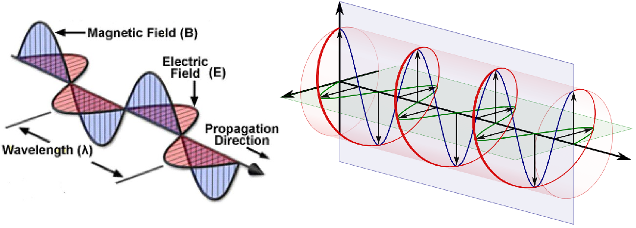
Fig. 23.1 Left Pane - Depiction of electric and magnetic plane waves, Right Pane - Depiction of electric and magnetic circularly polarised waves.

23.2. Polarisation of Waves

Plugging in wave solutions into Maxwell’s equations in vacuum:

(23.3)\[\begin{split}\nabla \cdot {\bf E} &= \,0 \Longrightarrow {\bf k} \cdot {\bf E}_0 = 0 \\ \nabla \cdot {\bf B} &= \,0 \Longrightarrow {\bf k} \cdot {\bf B}_0 = 0 \\ \nabla \times {\bf E} &= \,-\frac{\partial {\bf B}}{\partial t} \Longrightarrow {\bf k} \times {\bf E}_0 = \omega\, {\bf B}_0 \end{split}\]

These first two equations means \(\bf k \perp E\) and \(\bf k \perp B\) and the third that \(\bf B \perp (k,\, E)\) implying \(\bf E \perp B\).

Therefore once we pick a direction of oscillation for \(\bf E\), then \(\bf B\) is also set (and vice-versa). Choosing to orientate along the \(z\) axis, Equation (23.3) implies in general:

\[\begin{split}{\bf k} = \begin{bmatrix} 0 \\ 0 \\ k_z \end{bmatrix} \Longrightarrow {\bf E}_0 = \begin{bmatrix} E_x \\ E_y \\ 0 \end{bmatrix}\end{split}\]

For plane polarised solutions, we must pick one of \(E_x,\,E_y\) to be zero, such that the oscillations are only in on dimension and clearly the wave propagates in a perpendicular \(z\) dimension. So lets pick \(E_y = 0\), which results in:

(23.4)\[\begin{split}vE_0 = \begin{bmatrix} E_x \\ 0 \\ 0 \end{bmatrix} \Longrightarrow {\bf B}_0 = \frac{1}{\omega}({\bf k}\times {\bf E})= \begin{bmatrix} 0 \\ E_x \,k_z/\omega\\ 0 \end{bmatrix} = \begin{bmatrix} 0 \\ B_y \\ 0 \end{bmatrix} \end{split}\]

23.3. Drude Model

In addition to solving Maxwell’s for single electric charges, magnetic dipoles or in vacuum, we can also find other simple solutions. Within a conductor, with an electric field \({\bf E}\) present, we can think about Ohm’s law

\[V = I\,R\]

where \(V\) is the volatge applied over a conductor, \(I\) is the current flowing through a conductor and \(R\) is the electrical resitance. Each of these is potentially a variable - the resistiance of a condcutor can change depending on the length or cross-sectional area of the material. A better way to think about conductors and resitances is through the resisitivity \(\rho\):

\[\rho = R\frac{A}{\ell}\]

where \(R\) is the electrical resistance, \(\ell\) is the length of the conductor and \(A\) is the cross-sectional area of the condcutor, as depicted in Fig. 23.2.

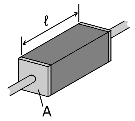
Fig. 23.2 A schematic of the geometry of some resistive material between some electrical contacts on both ends.

Thus we can rewrite Ohm’s law as:

\[V = \rho\,\frac{\ell\,I}{A} \Rightarrow \frac{I}{A} = \frac{1}{\rho}\frac{V}{\ell}\]

or terms of fields this is written:

\[{\bf J} = \sigma\, {\bf E}\]

where \(\sigma\) is the conductivity of the material, \(\rho = 1 / \sigma\) and \(\bf J\) is the current density. This is often known as the basis of the Drude Model of conductors.

Substituting this model into Maxwell’s equations, we can now source \(\bf J\) with this relation, if we choose to ignore free charges again \(\rho = 0\) and by solving for \(\bf E\):

\[\nabla^2 {\bf E} = \mu_0 \sigma \frac{\partial {\bf E}}{\partial t} + \mu_0\epsilon_0 \frac{\partial^2 {\bf E}}{\partial t^2}\]

Which should look familiar as a damped harmonic osciallator from the Waves section. Using the travelling wave solution ansatz, we find a dispersion relation of the form:

\[k^2 = \mu_0\epsilon_0\omega^2 + i \mu_0\sigma\omega\]

which is now in general complex!

We can rewrite this in the form of a relative permitivity \(\epsilon_r(\omega)\). Then we will take \(k^2 = \omega^2 / c^2 = \omega^2 \,\mu_0 \,\epsilon(\omega)\) with \(\epsilon = \epsilon_0\,\epsilon_r\) and so:

\[\epsilon_r(\omega) = \frac{\epsilon(\omega)}{\epsilon_0} = \underbrace{1}_{vacuum\, part} + \underbrace{i \frac{\sigma}{\epsilon_0\omega}}_{dispersion\,part} \]

If we calculate the energy of waves travelling through this media, the dispersion part corresponds to the energy losses of the electromagnetic field.

23.4. Electromagnetic Scalar and Vector Potentials

There is a different way to view Maxwell’s equations using the rules of vector calculus. We begin by expressing the electric field \({\bf E}\) in terms of a potential:

(23.5)\[{\bf E} = -\nabla \phi\]

where \(\phi = \phi(x,\,y,\,z)\) is the scalar electric potential. Gauss’s law \(\nabla\cdot {\bf E} = \rho/\epsilon_0\) means this now forms a Poisson equation:

\[\nabla^2\phi = -\frac{\rho}{\epsilon_0}\]

However the issue with Equation (23.5) is that it lacks are time dependence, which to solve Faraday’s law \(\nabla \times {\bf E} = -\partial {\bf B}/\partial t\) can cause issues:

\[\nabla \times {\bf E} = -\nabla \times \nabla \phi = 0 \]

where this result stems simply from vector calculus identities. Therefore in order to solve problems with time dependence, we must add a vector potential \({\bf A}\):

\[{\bf E} = -\nabla \phi - \frac{\partial {\bf A}}{\partial t}\]

Substituting this into Faraday’s law now results in:

\[\nabla \times {\bf E} = -\nabla \times \nabla \phi - \nabla \times \frac{\partial {\bf A}}{\partial t} = 0 - \frac{\partial}{\partial t}\left(\nabla \times {\bf A}\right) = - \frac{\partial {\bf B}}{\partial t}\]

which neatly suggests that:

\[{\bf B} = \nabla \times {\bf A}\]

which again through vector calculus identities satisfies \(\nabla \cdot {\bf B} = 0\). If we re-examine Gauss’s and Ampère’s law’s in light of these additions we find:

\[\begin{split}\nabla \cdot {\bf E} &=& \,-\frac{\partial}{\partial t}\left( \nabla \cdot {\bf A}\right) - \nabla^2\phi = \frac{\rho}{\epsilon_0}\\ \nabla \times {\bf B} &=&\, \nabla \left( \nabla \times {\bf A} \right) = \mu_0 {\bf J} + \mu_0 \epsilon_0 \frac{\partial {\bf E}}{\partial t} \\ &=& \,\mu_0 {\bf J} - \mu_0 \epsilon_0 \frac{\partial}{\partial t} \nabla \phi - \mu_0 \epsilon_0 \frac{\partial^2 {\bf A}}{\partial t^2}\end{split}\]

which we can rearrange, collect together terms and use vector identities to find a modified wave equation:

\[\frac{1}{c^2}\frac{\partial^2 {\bf A}}{\partial t^2} = \nabla^2 {\bf A} - \nabla \left(\nabla \cdot {\bf A} + \frac{1}{c^2}\frac{\partial \phi}{\partial t} \right) + \mu_0 {\bf J}\]

These two sets of equations are non-trivial to solve for \(\phi\) and \({\bf A}\). There are however a number of symmetries in this system of equations, one is that we can shift the parameters \(\phi,\,{\bf A}\) by functions of space and time and see what equations these should satisfy:

\[\begin{split}{\bf A} &\rightarrow&\, {\bf A} + \alpha({\bf x},\,t) \\ \phi &\rightarrow&\, \phi + f({\bf x},\,t)\end{split}\]

where \(f\) is a scalar shift and \(\alpha\) is a vector shift. If these shifts are to be symmetries of the electromagnetic equations, then they should NOT change the electric and magnetic fields overall, which means that:

\[\begin{split}{\bf E} & \rightarrow& -\frac{\partial}{\partial t}\left( {\bf A} + \alpha\right) - \nabla(\phi + f) = {\bf E} - \frac{\partial \alpha}{\partial t} - \nabla f \\ {\bf B} & \rightarrow& \nabla \times \left( {\bf A} + \alpha\right) = \nabla {\bf A} + \nabla \times \alpha = {\bf B} + \nabla \times \alpha \end{split}\]

and hence for unchanged fields, we must simultaneously satisfy:

\[\begin{split}\nabla \times \alpha &=&\, 0 \\ \frac{\partial \alpha}{\partial t} + \nabla f &=&\, 0\end{split}\]

Given that we can write an vector field with vanishing curl as a gradient of a scalar,

\[\alpha = \nabla \lambda\]

this means our second condition has the form

\[\nabla f = -\frac{\partial \alpha}{\partial t} = -\nabla \left(\frac{\partial \lambda}{\partial t} \right)\]

which we can rewrite our initial transformations in terms of

\[\begin{split}{\bf A} & \rightarrow&\, {\bf A} + \nabla \lambda\\ \phi &\rightarrow&\, \phi - \frac{\partial \lambda}{\partial t}\end{split}\]

Despite these transformations leaving \({\bf E},\,{\bf B}\) unchanged, the equations for Gauss’s and Ampères law are not invariant, since \(\nabla \cdot {\bf A}\) is still unconstrained. Thus we can use different choices of \(\phi\) and \({\bf A}\) here to simplify solving these. These different choices are known as Gauge Choices.

Writing electromagnetism in this way allows for quantum ideas and conceptual issues within these theories to be seen as physical effects, one way these are seen physically is through the Aharonov-Bohm (AB) effect. For more information on the AB effect, check out these DAMTP notes.