8. Energy and Power of Travelling Waves

8.1. Longitundinal wave energy and power

Given that waves are a method of propogating energy, it is an important question to ask how much and what parameters does a waves energy depend on!

Lets look at the total energy \(E\):

\[E = KE + PE\]

where \(KE\) is the total kinetic energy and \(PE\) the total potential energy.

Going back to the masses and springs model, the potential energy of each mass shown in Fig. 4.1 would be:

\[PE = \dots + \frac{1}{2}k\Big[u(x+h,t) - u(x,t)\Big]^2 + \frac{1}{2}k\Big[u(x+2h,t) - u(x+h,t)\Big]^2 + \dots\]

where each of the springs in the chain will contribute to the PE of two masses, depending on their orientation. Notice here that there are not any terms like \(PE \sim \frac{1}{2}k u^2(x,t)\), this is because we haven’t considered the effects at either end of the chain - although these edge effects are really important in real world systems, we will omit them here.

Using the springs in series result from (4.2), we can rewrite the PE in the form:

\[PE = \frac{1}{2}\,N\,k_{tot} \left(\dots + \Big[u(x+h,t) - u(x,t)\Big]^2 + \Big[u(x+2h,t) - u(x+h,t)\Big]^2 + \dots \right)\]

and likewise if we introduce the size of the mass \(m\) and then consider the total chain mass:

\[\begin{split}PE &= \frac{1}{2}\frac{N\,k_{tot}\,m}{m}\left(\dots + \Big[u(x+h,t) - u(x,t)\Big]^2 + \Big[u(x+2h,t) - u(x+h,t)\Big]^2 + \dots \right) \\ &= \frac{1}{2}\,m\frac{N^2\,k_{tot}}{m_{tot}}\left(\dots + \Big[u(x+h,t) - u(x,t)\Big]^2 + \Big[u(x+2h,t) - u(x+h,t)\Big]^2 + \dots \right)\end{split}\]

and then looking at the total chain length \(L = N\,h\):

\[PE = \frac{1}{2}\,m\,\frac{L^2\,k_{tot}}{m_{tot} h^2}\left(\dots + \Big[u(x+h,t) - u(x,t)\Big]^2 + \Big[u(x+2h,t) - u(x+h,t)\Big]^2 + \dots \right)\]

We recongise the term \(c^2 = L^2\,k_{tot}/m_{tot}\) and as before by taking the limit of \(N \rightarrow \infty \Rightarrow h \rightarrow 0\):

\[PE = \frac{1}{2}\,m\,c^2\,\lim_{h \rightarrow 0}\left(\dots + \Big[\frac{u(x+h,t) - u(x,t)}{h}\Big]^2 + \Big[\frac{u(x+2h,t) - u(x+h,t)}{h}\Big]^2 + \dots \right)\]

and (2.1) tells us that each of these limits corresponds to a partial derivative, thus:

\[PE = \frac{1}{2}\,m\,c^2\,\left(\dots + \Big[\frac{\partial}{\partial x}u(x+h,t)\Big]^2 + \Big[\frac{\partial}{\partial x}u(x+2h,t)\Big]^2 + \dots \right)\]

Likewise the kinetic energy has the form:

\[KE = \dots + \frac{1}{2}m\Big[\frac{\partial}{\partial t}u(x,t)\Big]^2 + \frac{1}{2}m\Big[\frac{\partial}{\partial t}u(x+h,t)\Big]^2 + \frac{1}{2}m\Big[\frac{\partial}{\partial t}u(x+2h,t)\Big]^2 + \dots\]

and so the total energy has the form:

\[E = \frac{1}{2}\,m\,\left(\dots + c^2\Big[\frac{\partial}{\partial x}u(x+h,t)\Big]^2 + \Big[\frac{\partial}{\partial t}u(x+h,t)\Big]^2 +\dots \right)\]

We can think of this system as a coupled harmonic oscillator, with each mass having oscillating \(KE\) and \(PE\) but the result from (3.2) tell us that the total amount of energy for each mass is fixed, so by symmetry over the whole chain we can simplify this to:

\[E = \frac{1}{2}\,m\,N\,\left[c^2\left(\frac{\partial u}{\partial x} \right)^2 + \left(\frac{\partial u}{\partial t} \right)^2\right] = \frac{1}{2}\,m_{tot}\,\left[c^2\left(\frac{\partial u}{\partial x} \right)^2 + \left(\frac{\partial u}{\partial t} \right)^2\right]\]

sometimes this is more usefully presented in terms of the energy per unit length or energy density \(\epsilon(x,\,t)\):

(8.1)\[\begin{split}\epsilon(x,\,t) = \frac{E}{L} &= \frac{1}{2}\,\frac{m_{tot}}{L}\,\left[c^2\left(\frac{\partial u}{\partial x} \right)^2 + \left(\frac{\partial u}{\partial t} \right)^2\right]\\ &= \frac{1}{2}\,\rho_L\,\left[c^2\left(\frac{\partial u}{\partial x} \right)^2 + \left(\frac{\partial u}{\partial t} \right)^2\right]\end{split}\]

where \(\rho_L\) is the mass per unit length or mass density of the mass and spring chain.

We can use this expression to find the total energy transferred over a wavelength:

(8.2)\[E_\lambda = \int_0^\lambda \epsilon(x,\,t) \,\mathrm{d}x \]

Likewise to find the power or rate of energy flow over a wave, we can use the definition of power:

\[P = \frac{\partial E}{\partial t}\]

In order to get a sensible physical quantity, we can find the time varying power:

(8.3)\[P(x,\,t) = \frac{\partial}{\partial t}\left(\int \epsilon(x,\,t) \,\mathrm{d}x\right) = \int \frac{\partial \epsilon}{\partial t} \,\mathrm{d}x \]

and then average the power over the time period \(T\), using the definition for the average value of a function:

(8.4)\[\langle P \rangle_T = \frac{1}{T}\int_0^T P(x,\,t) \,\mathrm{d}t \]

8.2. Transverse wave energy

Looking at the change total energy \(E\):

\[\Delta E = \Delta K + \Delta U\]

where \(K\) is the total kinetic energy and \(U\) the total potential energy.

\[\begin{split}\Delta K &= \frac{1}{2}\,\Delta m\,v^2 = \frac{1}{2}\,\rho_L\,\Delta x\, \left(\sqrt{1 + \left(\frac{\partial y}{\partial x}\right)^2}\right)\left(\frac{\partial y}{\partial t}\right)^2 \\ \Delta U &= T(\Delta s - \Delta x) = T\,\Delta x\,\left(\sqrt{1 + \left(\frac{\partial y}{\partial x}\right)^2} - 1\right)\end{split}\]

Recall for transverse waves \(\theta \ll 1\), therefore \(\partial y/\partial x \ll 1\) and so we can do a binomial expansion:

\[\begin{split}\Delta K &\simeq \frac{1}{2}\,\rho_L\,\Delta x\,\left(\frac{\partial y}{\partial t}\right)^2 + \dots, \\ \Delta U &\simeq T\,\Delta x\,\left(\frac{1}{2}\right)\left(\frac{\partial y}{\partial x}\right)^2 + \dots\\ \Rightarrow \Delta E &= \frac{1}{2} x\,\rho_L\,\left(\left(\frac{\partial y}{\partial t}\right)^2 + \frac{T}{\rho_L}\left(\frac{\partial y}{\partial x}\right)^2\right)\end{split}\]

and given that \(T / \rho_L = c^2\), we can simplify:

\[\Delta E = \frac{1}{2}\Delta x\,\rho_L\,\left[\left(\frac{\partial y}{\partial t}\right)^2 + c^2 \left(\frac{\partial y}{\partial x}\right)^2\right]\]

If we take the limit \(\Delta x \rightarrow 0\), then we can integrate up to find:

\[\int_0^E \textrm{d}E' = E = \int_0^\lambda \epsilon(x,t) \,\textrm{d}x \]

\[\epsilon(x,\,t) = \frac{1}{2}\,\rho_L\,\left[\left(\frac{\partial y}{\partial t}\right)^2 + c^2 \left(\frac{\partial y}{\partial x}\right)^2\right]\]

and we notice again the energy density term \(\epsilon(x,\,t)\), which matches that for longitundinal waves from Equation (8.1).

If we are deadling with waves propagating in two or three dimensions, with \(y = y({\bf x},\, t)\) then we can switch to using the gradient operator \(\nabla y\):

\[\epsilon({\bf x},\,t) = \frac{1}{2}\,\rho_L\,\left[\left(\frac{\partial y}{\partial t}\right)^2 + c^2 |\nabla y|^2\right]\]

8.3. Calculating the energy and power

Lets again start with a travelling wave \(u\):

\[u(x,\,t) = \mathrm{Re}\Big[u_0\, \exp\left(i(kx - \omega t)\right)\Big] = u_0\,\cos\left(kx - \omega t\right)\]

the energy density will be given by:

\[\begin{split}\epsilon &= \frac{1}{2}\,\rho_L\,\left[c^2\left(\frac{\partial u}{\partial x} \right)^2 + \left(\frac{\partial u}{\partial t} \right)^2\right] \\ &= \frac{1}{2}\,\rho_L\,{u_0}^2\,\sin^2\left(kx - \omega t\right)\left[c^2 k^2 + \omega^2 \right]\end{split}\]

and since \(\omega^2 = c^2\,k^2\) for travelling waves, this simplifies to:

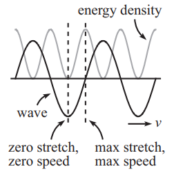
(8.5)\[\epsilon = \rho_L\,{u_0}^2\,\omega^2\,\sin^2\left(kx - \omega t\right)\]

Fig. 8.1 shows the difference in phase between \(u(x,\,t)\) and \(\epsilon(x,\,t)\).

Fig. 8.1 Breakdown of a travelling wave \(u(x,\,t)\) and the associated energy density \(\epsilon(x,\,t)\)

Calculating the energy carried over one wavelength:

\[\begin{split}E_\lambda &= \int_0^\lambda \rho_L\,{u_0}^2\,\omega^2\,\sin^2\left(kx - \omega t\right)\,\mathrm{d}x \\ &= \frac{1}{2}\rho_L\,{u_0}^2\,\omega^2\,\int_0^\lambda \left[1 - \cos\left(2kx - 2\omega t\right)\right]\,\mathrm{d}x\end{split}\]

where the second step used a double angle trigonometric identity to evaluate the integral:

\[\begin{split}E_\lambda &= \frac{1}{2}\rho_L\,{u_0}^2\,\omega^2\,\left[x - \frac{1}{2k}\sin\left(2kx - 2\omega t\right)\right]_0^\lambda \\ &= \frac{1}{2}\rho_L\,{u_0}^2\,\omega^2\,\left(\lambda - \frac{1}{2k}\sin\left(4\pi - 2\omega t\right) - 0 + \frac{1}{2k}\sin\left(- 2\omega t\right)\right)\end{split}\]

and we use \(k\lambda = 2\pi\) and by the cyclic nature of \(\sin(x)\), these terms cancel, leaving:

(8.6)\[E_\lambda =\frac{1}{2}\rho_L\,{u_0}^2\,\omega^2\,\lambda = \pi \,c^2\,\rho_L\,k\,{u_0}^2\]

Which suggests \(E_\lambda \propto {u_0}^2\), which is a key result.

Also note that if we did the same analysis with a left travelling wave \(u = u_0\,\exp(i(|k|x + |\omega|\,t))\), the result of Equation (8.5) would be the same.

Our analysis shows that for travelling waves with linear dispersion relation, the expression for \(\epsilon\) can be simplifed:

\[\epsilon = \rho_L\,c^2\,\left(\frac{\partial u}{\partial x} \right)^2 = \rho_L\,\left(\frac{\partial u}{\partial t} \right)^2\]

Note - this is simplified expression not true for waves with non-linear dispersion relations.

Likewise the wave power here comes out to be:

\[\begin{split}P(x,\,t) &= \int \frac{\partial \epsilon}{\partial t} \,\mathrm{d}x = 2\rho_L\,{u_0}^2\,\omega^3\,\int\sin\left(kx - \omega t\right)\cos\left(kx - \omega t\right)\,\mathrm{d}x \\ &= \frac{1}{k}\rho_L\,{u_0}^2\,\omega^3\,\sin^2\left(kx - \omega t\right) = \rho_L\,{u_0}^2\,\omega^2\,c\,\sin^2\left(kx - \omega t\right)\end{split}\]

Notice that this result is related to (8.5) by \(P = c\,\epsilon\).

In order to make sense of the power however, we need to average it over the time period, which is:

\[\begin{split}\langle P \rangle_T &= \frac{1}{T}\int_0^T P(x,\,t) \,\mathrm{d}t = \frac{1}{T}\,\rho_L\,{u_0}^2\,\omega^2\,c\,\int_0^T \sin^2\left(kx - \omega t\right)\,\mathrm{d}t \\ &= \frac{\rho_L\,{u_0}^2\,\omega^2\,c}{2T}\,\int_0^T \left(1 - \cos\left(2kx - 2\omega t\right)\right)\,\mathrm{d}t \\ &= \frac{\rho_L\,{u_0}^2\,\omega^2\,c}{2T}\,\Big[t + \frac{1}{2\omega}\sin\left(2kx - 2\omega t\right)\Big]_0^T \\ &= \frac{\rho_L\,{u_0}^2\,\omega^2\,c}{2T}\,\Big(T + \frac{1}{2\omega}\sin(2kx - 4\pi) - 0 - \frac{1}{2\omega}\sin(2kx)\Big)\end{split}\]

where we use \(\omega T = 2\pi\) and by the cyclic nature of \(\cos(x)\), these terms cancel, leaving:

\[\langle P \rangle_T = \frac{1}{2}\rho_L\,\omega^2\,c\,{u_0}^2 = \frac{1}{2}\rho_L\,c^3\,k^2\,{u_0}^2\]

and here we see that \(\langle P \rangle_T\propto {u_0}^2\).

If we think back to oscilating electrical systems, for an oscillating voltage \(v = V_0\cos(\Omega t)\), the electrical power would be \(P = V^2 / R = {V_0}^2\,\cos^2(\Omega t)/R\) - suggesting the power and oscillation amplitude are related according to \(P \propto {V_0}^2\), which we see is a general fact of oscillating systems.