7. Dispersion Relations and Wave Speed

7.1. Dispersion relation

Now that we have our complex wave solutions to the equation, we can see that plugging in the solutions to the wave equation produce their own equations. Lets start with the simplest wave solution, a 1D right hand moving wave:

(7.1)\[u = u_0\,\exp(i(kx-\omega t))\]

Plugging this into the wave equation:

\[\begin{split}u_{xx} &= \,-k^2 \,u\\ u_{tt} &= \, -\omega^2 \,u \\ u_{tt} &= \, c^2\,u_{xx} \\ -\omega^2 \,u &= \, -c^2\,k^2\,u \Rightarrow \omega^2 &=& \,c^2 k^2 \Rightarrow \omega = \,\pm\, c k\end{split}\]

Since we have two roots for \(\omega\) here, we can see that these correspond to either left or right hand moving waves.
Therefore if we use (7.1) with the proviso that \(\omega = \omega(k) = \pm c\, k\), this describes the d’Alembert wave solutions.

The function \(\omega = \omega(k)\) is known as a dispersion relation. In this case, \(\omega(k)\) is a linear function of \(k\), but in general it could be any function of \(k\). We can also rewrite this linear expression in terms of frequency and wavelegnth \(f = \omega/2\pi, \,\lambda = 2\pi/k\):

\[c = f \,\lambda\]

which is of course a familiar result!

We do not in general need to stick to \(\omega = c\,k\) however, as we will see later, non-linear dispersion relations are not uncommon and result from have a different form of wave equation.

Looking at the combination of \(\omega/k\), notice it has units of:

\[\frac{[\omega]}{[k]} = \frac{s^{-1}}{m^{-1}} = m\,s^{-1} = [\textrm{speed}]\]

and so we see this is a wave speed of some sort!

7.2. Group and Phase Velocity

We can start by considering again the movement of waves in time and space:

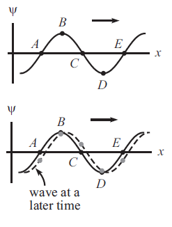
Fig. 7.1 Visulisation of a wave moving in time and space.

A solution for these waves, \(u(x,\,t) = u_0\,\cos(kx-\omega t)\), shows that although \(x,\,t\) vary, each part of the waves remain a fixed distance apart - this is the wave phase \(\Phi = kx - \omega t\). Therefore this wave phase is invariant in space and time, hence:

\[\frac{\partial \Phi}{\partial t} = k\frac{\partial(x)}{\partial t} - \omega = 0\]

which we can rearrange to find:

\[v = \frac{\partial(x)}{\partial t} = \frac{\omega}{k}\]

This is known as the phase velocity of the wave \(v_p\) and describes the rate at which the phase of the wave propagates through space.

However this measure of wave velocity is only really unambiguous if there is a single wave moving in space and time, what happens if we have multiple waves?

Lets consider a sum of two waves, of equal amplitude, but different frequencies and wavelengths:

\[u = u_1 + u_2 = u_0\cos(k_1x-\omega_1t) + u_0\cos(k_2x - \omega_2t)\]

we can rewrite this using trigonometric identities:

\[\begin{split}\cos(A+B) &= \cos(A)\cos(B) - \sin(A)\sin(B) \\ \cos(A-B) &= \cos(A)\cos(B) + \sin(A)\sin(B) \\ \Rightarrow \cos(A+B) + \cos(A-B) &= 2\cos(A)\cos(B) \\ \Rightarrow \cos(C) + \cos(D) &= 2\cos\left(\frac{C+D}{2}\right)\,\cos\left(\frac{C-D}{2}\right)\end{split}\]

So we can rewrite our superposition of two waves as:

\[u = 2u_0\,\cos\left(k_{avg}\,x - \omega_{avg}\,t\right)\,\cos\left(\frac{\Delta k}{2}x - \frac{\Delta \omega}{2}t\right)\]

where we have defined:

\[\begin{split}k_{avg} = \frac{k_1+k_2}{2} &\qquad \omega_{avg} = \frac{\omega_1+\omega_2}{2} \\ \Delta k = k_1-k_2 &\qquad \Delta \omega = \omega_1-\omega_2 \end{split}\]

Equally we could do this in the complex representation:

\[\begin{split}u &= u_0\,\exp\left[i(k_1x-\omega_1t)\right] + u_0\,\exp\left[i(k_2x-\omega_2t)\right] \\ &= u_0\exp\left[i\left(\frac{k_1+k_2}{2}x - \frac{\omega_1+\omega_2}{2}t\right)\right]\,\exp\left[i\left(\frac{k_1-k_2}{2}x - \frac{\omega_1-\omega_2}{2}t\right)\right]\\ &= u_0\exp\left[i(k_{avg}\,x - \omega_{avg}\,t)\right]\,\exp\left[i\left(\frac{\Delta k}{2}x - \frac{\Delta \omega}{2}t\right)\right]\end{split}\]

The result of this can be visualised in Fig. 7.2

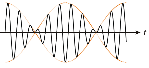
Fig. 7.2 Visulisation of a superposition of two waves moving in time and space, the result is known as beats where wave follows an outer envelope function (dashed line), even though the overall phase (the black line) remains fixed.

We can track the phase of the waves now with the first cosine term, which we see follows:

\[\begin{split}\Phi_1 &= k_{avg}\,x - \omega_{avg}\,t \\ \Rightarrow \frac{\partial x}{\partial t} &= v_p = \frac{\omega_{avg}}{k_{avg}}\end{split}\]

but the combined wave moves as a group, signified by the second cosine term:

\[\begin{split}\Phi_2 &= \frac{\Delta k}{2}\,x - \frac{\Delta \omega}{2}\,t\\ \Rightarrow \frac{\partial x}{\partial t} &= v = \frac{\Delta \omega}{\Delta k}\end{split}\]

If we pick a continuum of waves, then in the limit of \(\Delta k \rightarrow 0\), each of the waves is separated by an infinitesimal difference \(\mathrm{d}k\), meaning:

\[v_g = \frac{\mathrm{d}\omega}{\mathrm{d}k}\]

This is known as the group velocity of the wave and describes the velocity with which the overall envelope shape of the wave’s amplitudes propagates through space and time. We also see that this velocity is dimensionally equivalent to \(v_p\).

We can see this effect of beats illustrated in figure Fig. 7.3.

Fig. 7.3 Two right travelling waves with slightly different frequencies/wavelengths, producing a beat wave.

We can extend this to two and higher dimensions using partial derivatives and the gradient operator:

\[\begin{split}\bf{v_p} &=& \,\frac{\bf \hat{k} }{|\bf{k}|}\omega \\ \bf{v_g} &=& \,\nabla_k \,\omega \end{split}\]

Usually these vectors point in the same direction, but there are examples in nature, for instance the anisotropic structure within a crystal, where the two vectors are not parallel.

7.3. Non-linear dispersion relation and wave speeds

The first thing to notice about the phase and group velocities is that for a linear dispersion relation, they are equal:

\[\begin{split}\omega &= ck\\ v_p &= \frac{\omega}{k} = c \\ v_g &= \frac{\mathrm{d}\omega}{\mathrm{d}k} = c\end{split}\]

However once we look at non-linear \(\omega(k)\) then the picture changes. Lets look at a power law type dispersion relation:

\[\omega = A k^{r}\]

where \(A\) is a constant that has units of \([A] = s^{-1}\,m^{r}\) and \(r\) is some constant exponent to be chosen.

There will be different regimes of \(r\) values of interest:

1. \(0 < r < 1\)

This is non-linear dispersion relation:

\[\begin{split}v_p &= \frac{\omega}{k} = Ak^{r-1} \\ v_g &= \frac{\mathrm{d}\omega}{\mathrm{d}k} = Ark^{r-1}\end{split}\]

and since \(r<1\), \(v_g < v_p\), which means that the wave envelope is moving slower than the individual parts of the wave.

2. \(r=1\)

This is linear dispersion relation:

\[\begin{split}v_p &= \frac{\omega}{k} = A \\ v_g &= \frac{\mathrm{d}\omega}{\mathrm{d}k} = A\end{split}\]

and so \(v_g = v_p\), which means that all parts of the wave are moving at the same speed.

3. \(r > 1\)

This is non-linear dispersion relation:

\[\begin{split}v_p &= \frac{\omega}{k} = Ak^{r-1} \\ v_g &= \frac{\mathrm{d}\omega}{\mathrm{d}k} = Ark^{r-1}\end{split}\]

and since \(r>1\), \(v_g > v_p\), which means that the wave envelope is moving faster than the individual parts of the wave.

We can see these cases summarised in Fig. 7.4.

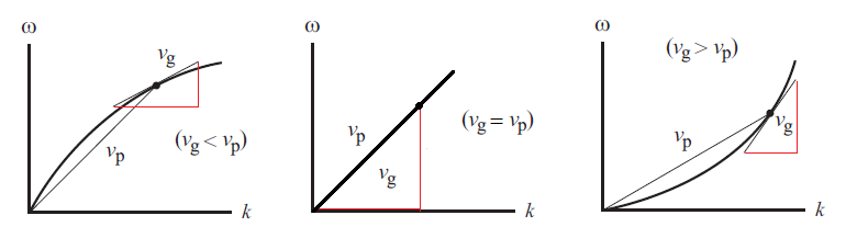
Fig. 7.4 Visualisation of the differences between phase and group velocity in the case of a power law dispersion relation. The left hand figure shows \(r < 1\), the middle figure shows \(r = 1\) and the right hand figure shows \(r > 1\).

What about more radical choices of dispersion relation, we could even make this some kind of inverse relationship:

4. \(r < 0\),

Here lets say \(\displaystyle A = \frac{A}{k^{r}}\), then: Here lets say \(\displaystyle A = \frac{A}{k^{r}}\), then:

\[\begin{split}v_p &= \frac{\omega}{k} = \frac{A}{k^{r+1}} \\ v_g &= \frac{\mathrm{d}\omega}{\mathrm{d}k} = -\frac{Ar}{k^{r+1}} \end{split}\]

i.e. \(v_g = -r v_p\), which is quite dramatic, it suggests that the wave envelope is moving in the opposite direction to the individual parts of the wave! We can illustrate this in an \(\omega-k\) plot in Fig. 7.5.

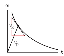
Fig. 7.5 Visualisation of the differences between phase and group velocity in the case of a power law dispersion relation \(\displaystyle \omega = \frac{A}{k^r}\). Note that this shows \(v_g = -r v_p\).

7.4. Wavepackets

Our simplest form of dispersion relation for travelling waves suggested \(\omega = \pm ck\), which we can write as:

\[\begin{split}u(x,\, t) &=\, \sum_{n=1}^2 u_n \exp(i(kx-\omega_n t))\\ \omega_n &=\, (-1)^n\,ck \end{split}\]

where \(u_n\) is a each waves amplitude. We can generalise this by letting \(u_n = u_n(k)\) and using a continuous spectrum of \(k\) values with a general dispersion relation \(\omega = \omega(k)\), therefore:

\[u(x,\, t) = \int^{\infty}_{-\infty} A(k) \,\exp(i(kx-\omega(k)t))\,\mathrm{d} k\]

We call these wave packets, also known sometimes as wave trains or bursts - we can picture them as a larger wave envelope, with smaller localized waves that travel as one unit together, as shown in Fig. 7.6. This infinite set of oscillating waves have different wavelengths, with phases and amplitudes that constructively and destructively interfereonly over different regions of space.

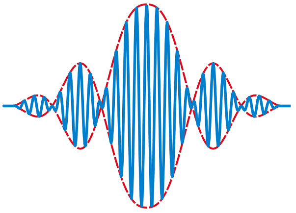
Fig. 7.6 Schematic of a wave packet, with localisation near the centre of the packet.

Each component wave here is a solution of a wave equation and so the entire wave packet is. Depending on the wave equation, the wave packet’s profile may remain constant (no dispersion) or change (dispersion) while propagating.

These can help us understand the differences between group and phase velocity, as outlined in Fig. 7.7

Fig. 7.7 A wave packets showing key differences between group and phase velcoities.

7.4.1. Dispersion-less wavepackets

Here although the wave is a superposition of many waves, they follow a linear dispersion relation \(\omega = ck\), meaning phase and group velocity are the same and so the waves travel as one complete train, as seen in figure Fig. 7.8.

Fig. 7.8 A wave packet moving in a dispersion-less medium.

7.4.2. Dispersive wavepackets

Here in addition to the wave is a superposition of many waves, they follow a non-linear dispersion relation \(\omega = \omega(k)\) where phase and group velocities differ and the waves travel as a train which begins to spread as it travels, as seen in figure Fig. 7.9.

Fig. 7.9 A wave packet moving in a dispersive medium.