1. Mathematical Prelimaries¶

1.1. Set Theory¶

Set theory is a branch of mathematics that studies collections of objects known as Sets. The language of set theory, which will start to study here, can be used to define almost all mathematical objects (if you are interested in what cannot be so easily defined, look up ideas such as Gödel’s incompleteness theorem and Russell’s Paradox).

1.2. Notation¶

There are lots of symbols in the notation used to describe mathematical objects, some of which we may have seen already. We can put together some elementary operations on sets:

Symbol	Meaning	Example
\(\{ \}\)	Defines a set	e.g. \(A = \{1,\,2,\,3,\,4\}\), \( B = \{3,\,4,\,5\}\)
\(A \cup B\)	Union - in \(A\) OR \(B\) (OR both)	\(A \cup B = \{1, \,2, \,3, \,4, \,5\}\)
\(A \cap B\)	Intersection - in \(A\) AND \(B\)	\(A \cap B = \{3, \,4\}\)
\(A \subseteq B\)	Subset - every element of \(A\) is in \(B\)	\(\{3,\,4,\,5\} \subseteq B\)
\(A \subset B\)	Proper Subset - every element of \(A\) is in \(B\), but \(B\) has more elements	\(\{1,\, 2,\, 3\} \subset A\)
\(A \not\subset B\)	Not a Subset - \(A\) is not a subset of \(B\)	\(\{1, \,5\} \not\subset A\)

Additionally we can build up structure with some more advanced operations on sets:

Symbol	Meaning	Example
\(\varnothing\)	Empty set \( = \{\}\)	\(\{1,\, 2\} \cap \{3,\, 4\} = \varnothing \)
\(\mathbb{U}\)	Universal Set - set of all possible values in the area of interest	e.g. \(\mathbb{U} = \{1,\,2,\,3,\,4,\,5,\,6,\,7\}\)
\(A^c\) or \(A'\) or \(\neg A\) or \(\bar{A}\)	Complement - elements not in \(A\)	\(\neg A = \{5,\,6,\,7\}\) \(B' = \{1,\, 2, \,6,\, 7\}\)
\(a \in A\)	Element of - \(a\) is in \(A\)	\(3 \in A\)
\(b \notin A\)	Not element of - \(b\) is not in \(A\)	\(6 \notin A\)
\(A = B\)	Equality - both sets have the same members	e.g. \(C = \{5,\,3,\,4\},\, C = B\)
\(A \times B\)	Cartesian Product - set of ordered pairs from \(A\) and \(B\)	\(\{1,\, 2\} \times \{3, \,4\} \) \(= \{(1, \,3), \,(1,\, 4), \,(2,\, 3),\, (2,\, 4)\}\)
\(\\|A\\|\) or \(n(A)\)	Cardinality - the number of elements in set \(A\)	\(\\|A\\| = 4,\,\\|B\\| = 3\)
\(\\|\) or \(:\) or st	Such that	\(\{ n\, \\|\, n > 0 \} = \{1, 2, 3, \dots\}\)
\( \forall\)	For All	\(\forall \,x > 1,\, x^2 > x\)
\(\exists\)	There Exists	\(\exists \, x \,\\|\, x^2 > x\)
\( \therefore\)	Therefore	\( a = b \therefore b=a\)
iff or \(\iff\)	If and only if	\(2a = 2\) iff \(a=1\)

1.3. Definition of a set¶

There are two basic ways to define a set:

List / Tabular Form, where we list the members of the set in any order. For example, the set of all the vowels and consonants:

\[\begin{split} V &= \{a,\,e,\,i\,o,\,u\} \\ C &= \{b,\,c,\,d,\,f,\,g,\,h,\,j,\,k,\,l,\,m,\,n,\,p,\,q,\,r,\,s,\,t,\,v,\,w,\,x,\,y,\,z\}\end{split}\]

or the set of the Natural number and Integers:

\[\begin{split} \mathbb{N} &= \{1,\,2,\,3,\dots \} \\ \mathbb{Z} &= \{ \dots,\,-3,\,-2,\,-1,\,0,\,1,\,2,\,3,\,\dots \}\end{split}\]

Set-Builder Form / Property Method, where we state the properties which characterise the elements of a set, i.e. those held by members of the set (but not by non-members. For example:

\[ A = \{x\,:\, x \text{ is an integer}\}\]

which we read is ”The set \(A\), defined by elements \(x\), such that \(x\) is an integer”. There are many ways to write out such a statement, the simplest is to use the wider notation of set theory. For example, the set of Rational numbers or Complex numbers:

\[\begin{split} \mathbb{Q} &= \left\{ \frac{m}{n} \,\,\middle|\,\, m,\,n \in \mathbb{Z}\right\} \\ \mathbb{C} &= \left\{ a + i\,b \,\,\middle|\,\, a,\,b\in \mathbb{R},\, i^2 = -1\right\}\end{split}\]

1.4. Functions¶

We are probably quite used to thinking about functions when we plot graphs, such as \(y = x^2\) or \(y = \cos(x)\), as we idealise in Fig. 1.1.

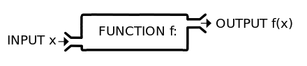
Fig. 1.1 These are examples of a much richer mathematical structure, known as Functions, which we can roughly think of as a machine with inputs and outputs.¶

1.4.1. Definition of a Function¶

To set this up in a firmer mathematical way, we can think about functions as the mapping of elements between different sets. Lets denote the set \(A\), which contain the elements we wish to map unique to elements in another set \(B\), this mapping will be the function \(f\) from \(A\) to \(B\):

\[f:\,A \rightarrow B\]

which we read as “\(f\) is a function from \(A\) to \(B\)”. The elements of the set \(A\), which we think of as the range of values in the inputs, is known as the Domain of the function and elements of the set \(B\), which we think of as the range of values of the outputs are known as the Target Set or Co-Domain of the function.

There are several notations for functions:

Notation	Meaning
\(f(x) = x^2\)	\(x\) as a variable for the function \(f\)
\(x \mapsto x^2\)	\(x\) goes into \(x^2\)
\(y = x^2\)	\(x\) is the independent variable and & \(y\) is the dependent variable

Given a function \(f:\, A \rightarrow B\), then for an element \(a \in A\) the function \(f(a)\) maps \(a\) to a unique element in \(b \in B\).

We call \(f(a)\) the Image of \(a\) under \(f\), or \(d(a)\) is the Value of \(f\) at \(a\) or that \(f\) Sends or Maps \(a\) into \(f(a)\).

The set of all image values is called the Range or Image of \(f\), which is denoted as:

\[ \text{Im}(f) = \text{Ran}(f) = f(A) = \{b \in B\,:\, \text{there exists }\, a \in A \,\,\text{for which }\, f(a) = b\}\]

and we should make clear that \(\text{Im}(f) \subset B\).

Given \(f: A \rightarrow B\), then for some subset \(A' \subset A\). \(f(A')\) denotes the set of images of elements in \(A'\) and if \(B' \subset B\) and \(f^{-1}(B')\) denotes the set of elements of A each whose image belongs to \(B'\):

\[ f(A') = \{f(a)\,:\,a \in A\} \Longleftrightarrow f^{-1}(B') = \{a\in A\,:\,f(a)\in B\}\]

given we call \(f(A')\) the imagine of \(A'\), we call \(f^{-1}(B')\) the Inverse Image or Preimage of \(B'\).

We also define an Identity function \(I_A\), which simply send an element back to itself, \(I_A:\,A \rightarrow A\):

\[I_A(a) = a\]

for every element \(a \in A\).

Finally we can define the Graph of a function \(f:\,A \rightarrow B\) as the series of order pairs of elements \(a \in A\) mapped to elements \(b = f(a) \in B\):

\[\text{Graph of }\,f = \{(a,\,b)\,:\, a \in A,\,b = f(a)\}\]

A function \(f\) is defined from a set \(A = \{a,\,b,\,c,\,d\}\) into a set \(B = \{r,\,s,\,t,\,u\}\). with a mapping:

\[\begin{split}f(a) &= s \\ f(b) &= u \\ f(c) &= r \\ f(d) &= s\end{split}\]

which we can represent graphically as shown in Fig. 1.2.

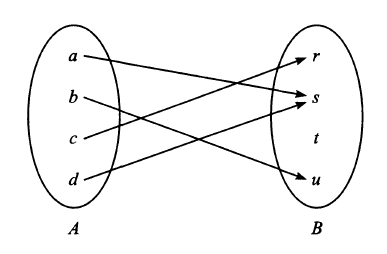
Fig. 1.2 The image \(f\) is the set \(\text{Im}(f) = \{r,\,s,\,u\}\) and the element is \(t \notin \text{Im}(f)\) because \(t\) is not the image of any element of \(A\) under \(f\) - therefore any elements not mapped to under a function are excluded from the image of the function.¶

The graph of \(f\) is the following set of ordered pairs:

\[\{ (a,\,s),\,(b,\,u),\,(c,\,r),\,(d,s) \}\]

1.5. Composite Functions¶

Using the idea of mapping from one set to another, it is possible to introduce functions of functions or composite functions, mapping from one set to another, through some intermediate set. Consider functions \(f:\,A \rightarrow B\) and \(g:\,B \rightarrow C\), where the target set \(B\) of \(f\) is the domain of \(g\). We can call this new function the Composition of \(f\) and \(g\), denoted by:

\[g \circ f \equiv g(f(a)\]

where we emphasise that the composition of functions is read from right to left (and not left to right as we usually do). We picture this in Fig. 1.3.

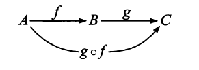
Fig. 1.3 We can introduce more and more functions and same rules apply, however we can also consider the associativity of the composition of functions, given \(f:\,A \rightarrow B,\,g:\, b \rightarrow C,\,h:\,c \rightarrow D\).¶

The composition law is also associative:

\[h \circ(g \circ f) = (h \circ g) \circ f\]

which we prove diagrammatically in Fig. 1.4.

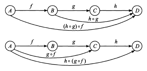
../_images/associativitycompositefunctions.png

Fig. 1.4 Associativity of composite functions.¶

Lets think about two simple functions:

\[\begin{split}f(x) &= x^2\\ g(x) &= \cos(x)\end{split}\]

We can composite these functions by writing:

\[\begin{split}f(g(x)) &= (f \circ g)(x) &= (\cos(x))^2 \\ g(f(x)) &= (g \circ f)(x) &= \cos(x^2)\end{split}\]

where we notice that in general \(f(g(x)) \neq g(f(x))\). These composite functions can be built up by looking at the function on the furthest right and then adding more functions on to the left hand side. Suppose we introduce a third function:

\[h(x) = \frac{2}{x}\]

then the six different functional compositions would be:

\[\begin{split}f \circ (g \circ h) &= \left( \cos \left( \frac{2}{x} \right) \right)^2 & f \circ (h \circ g) = \left( \frac{2}{\cos(x)} \right)^2 \\ g \circ (h \circ f) &= \cos \left( \frac{2}{x^2} \right) & g \circ (f \circ h) = \cos \left( \left( \frac{2}{x}\right)^2 \right) \\ h \circ (f \circ g) &= \frac{2}{\left( \cos (x) \right)^2 } & h \circ (g \circ f) = \frac{2}{\cos(x^2)}\end{split}\]

and we see that the associativity of these composites can be shown to be true:

\[\begin{split} f\circ g &= (\cos(x))^2\\ g \circ h &= \cos\left(\frac{2}{x}\right) \\ f \circ (g \circ h) &= (f \circ g) \circ h = \left( \cos \left( \frac{2}{x} \right) \right)^2\end{split}\]

1.6. Invertibility of Functions¶

A function \(f:\,A \rightarrow B\) is said to be one-to-one or Injective if different elements in the domain \(A\) have distinct images, i.e.

\[f\,\text{ is one-to-one if }\,f(a) = f(a') \Rightarrow a = a'\]

Likewise we can set up a function \(f:\,A \rightarrow B\) is said to be an onto function or Surjective if every element \(b \in B\) is the image of some element \(a \in A\), i.e. the image of \(f\) is the entire target set \(B\):

\[f\,\text{ maps }\,A \text{ onto }\,B\,\text{ if }\,\forall\, b \in B,\, \exists \,a \in A, \,\text{ s.t.}\, f(a) = b\]

A function \(f:\,A \rightarrow B\) is said to be invertible if there exists a function \(f^{-1}:\, B\rightarrow A\) such that:

\[f^{-1} \circ f = I_A \Longleftrightarrow f \circ f^{-1} = I_B\]

A function \(f:\,A \rightarrow B\) is invertible iff \(f\) is both one-to-one and onto. We say such functions are a one-to-one correspondence between \(A\) and \(B\). This is also known as a Bijection.

Lets consider functions \(f_1:\,A \rightarrow B\), \(f_2:\,B \rightarrow C\), \(f_3:\,C \rightarrow D\), \(f_4:\,D \rightarrow E\) depicted in Fig. 1.5

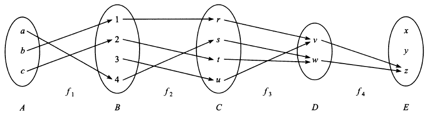
Fig. 1.5 Invertibility of four functions which map elements from \(A \rightarrow B \rightarrow C \rightarrow D \rightarrow E\).¶

\(f_1:\,A \rightarrow B\) is one-to-one but not onto, since every element in \(A\) has a unique image, but element \(3 \in B\) does not have any image under \(f_1\).
\(f_2:\,B \rightarrow C\) is both one-to-one and onto, i.e. it is a onto-to-one correspondence for all elements in \(B\) and \(C\) and thus \(f^{-1}:\, C \rightarrow B\) exists.
\(f_3:\,C \rightarrow D\) is not one-to-one but is onto since \(f_3(r) = f_3(u) = v\), but every element in \(D\) has an image under \(f_3\).
\(f_4:\, D \rightarrow E\) is neither one-to-one nor onto, since \(f_4(v) = f_4(w) = z\) and there are elements in \(E\) which are not images under \(f_4\).

Mathematics for Natural Sciences A

Mathematical Prelimaries

Contents