Limits of Functions and Sequences
Contents
4. Limits of Functions and Sequences
4.1. Limit of a function
The mathematics of limits are used to describe the behaviour of a function or sequence that is approaching a point, rather than being defined at it.
Worked Example 1
We start with a simple example, the function \(f(x) = x^2\) near to the point (2,4).
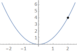
Fig. 4.1 A plot of \(f(x)=x^2\) together with the point \((2,4)\).
In this example, it is apparent that we can trace along the \(x^2\) curve towards the point, from either direction.
Mathematically, we say that we can make \(f(x)\) arbitrarily close (“as close as you like”) to 4 by making \(x\) sufficiently close to 2.
We write:
and we say that “the limit of \(x^2\) as \(x\) tends to (approaches) 2 is equal to 4”.
In fact, for the squared function, it is clear that
for all \(c\). However we will see that this behaviour does not apply for all functions.
We may also consider the limit of a function \(f(x)\) as its argument \(x\) becomes “very large”, for instance, we can say that
since \(x^2\) can be made arbitrarily large by making \(x\) “big enough”. We would read the expression by saying: “the limit of \(x^2\) as \(x\) tends to infinity is infinity”, though it does not actually reach infinity.
Worked Example 2
We can find functions which approach a finite value as \(x \to \infty\), and also functions which approach infinity whilst \(x\) remains finite.
For example, consider the behaviour of \(f(x) = \displaystyle\frac{1}{x}\),
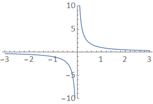
Fig. 4.2 A plot of \(f(x) = 1/x\).
In this case, as \(x\) becomes very large, \(f(x)\) approaches zero and so we can write:
The \(0^+\) and \(0^−\) have been used here to indicate that the function “tends to zero from above/below” as \(x\) tends to positive and negative infinity respectively. Likewise we see that:
4.1.1. Technical definition
Formally speaking the limit of a function \(\lim_{x \to c} f(x) = L\) is defined as for every real \(\epsilon > 0\), there exists a real \(\delta >0\) such that for all real \(x\),
Notice there that no part of the definition requires that the value of \(f(c)\) is defined. We can think of \(\epsilon\) as the error and \(\delta\) as the distance, such that the error in measuring that the value at the limit point \(c\) can be made as small as desired, by reducing the distance to the limit point.
4.2. The one-sided limit
We can motivate the idea of a one-sided limit from \(f(x) = \displaystyle\frac{1}{x}\), where:
Since the left and right limits are not the same, then we cannot meaningfully refer to the limit of this function without providing a direction, so the result for \(\displaystyle\lim_{x \to 0} \frac{1}{x}\) is undefined.
We would technically say that this function is discontinuous at \(x = 0\), although it is piecewise continuous on each of the pieces either side of \(x=0\), i.e. there is an interval over which it is continuous, just not over all \(x\) values.
Another example of a piecewise continous function is the Heaviside step function, which we define as:
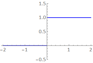
Fig. 4.3 A plot of the Heaviside function \(H(x)\).
We see that this function has a finite jump (or discontinuity) at \(x=0\) and therefore a one sided limit is needed for \(x = 0\).
4.3. Combination of limits
It is useful to know how to solve the limit of combinations of functions (or “functions of functions”), such as:
where \(c\) can be any value we wish to approach.
The approach we take to solve these depends on whether the limits of the inidividual functions \(\displaystyle\lim_{x \to c} f(x)\) and \(\displaystyle\lim_{x \to c} g(x)\) are finite or infinite.
4.3.1. Functions that tend to finite values
First consider the case where the limit of all the functions are finite. If and only if the limits of the individual functions are finite then we can use the combination theorem to solve the combination of functions.
Definition of the combination theorem
If the limits \(\displaystyle\lim_{x \to c} f(x)\) and \(\displaystyle\lim_{x \to c} g(x)\) are finite then the combination theorem tells us that:
1.
2.
where \(\alpha\) and \(\beta\) are constants. 3.
Note that the combination theorem for limits can only be used if the limit of every function is finite.
Worked Example
As an example, consider the function:
Since the limits of each of the individual functions are finite: \(\displaystyle\lim_{x \to 0} x^2 = 0\), \(\displaystyle\lim_{x \to 0} (x+1)^3 = 1\) and \(\displaystyle\lim_{x \to 0} (x-1)^3 = -1\), we can use first and third statment of the combination theorem to rewrite and solve the equation as:
4.3.2. Functions that tend to infinite values
We now consider the case where the limit of all the individual functions are infinite, such as \(\displaystyle\lim_{x\to \infty} x^2\) or \(\displaystyle\lim_{x\to 0^-} \frac{1}{x}\).
Warning!
As an example consider the funcion \(f(x) = x(x-1) = x^2 - x\):
This limit appears to “go like” \(\infty - \infty\), so you may think this result is zero - but it is not!
Generally speaking we should not treat \(\infty\) like a number.
There is a sense in which \(x^2\) is “much bigger” than \(x\) and so it dominates this expression - that is to say that \(x^2\) “blows up faster” than \(x\) as \(x\to \infty\).
This means that in this limit the difference between \(f(x) = x^2-x\) and a function \(g(x) = x^2\) becomes smaller and smaller as \(x\to \infty\).
Both of these functions however approach infinity in the limit of \(x\to \infty\):
Worked Example
Lets consider a function:
and look at the limit as \(x \to \infty\):
It can be tempting to consider this (pehaps using the combination theorem) as \(\displaystyle \frac{\infty}{\infty} = 1\), but as discussed we should not think of \(\infty\) as a number, only a limit.
To take these infinite limits, lets simplify the function first, but dividing through by \(x\) in the denominator and numerator:
and since \(\displaystyle\lim_{x\to\infty} \frac{1}{x} = \lim_{x\to\infty} \frac{2}{x^2} = 0\), the solution of the limit is \(\displaystyle \frac{1}{4}\).
Practice Questions
Find the following limits:
1. \(\displaystyle\lim_{x\to\infty} \frac{x+2}{x^2-2}\).
2. \(\displaystyle\lim_{x\to\infty} \frac{x-2}{x+2}\).
3. \(\displaystyle\lim_{x \to \infty} \big( \sqrt{x^2-2} - \sqrt{x^2+x} \big)\).
Solutions
1. \(\displaystyle\lim_{x \to \infty}\frac{x+2}{x^2 - 2} = \lim_{x \to \infty} \frac{1/x + 2/x^2}{1-2/x^2} = \frac{0+0}{1+0} = 0\).
2. \(\displaystyle\lim_{x \to \infty}\frac{x-2}{x+2} = \lim_{x \to \infty} \frac{1 - 2/x}{1+2/x}= \frac{1-0}{1+0} = 1\).
3. Firstly we need to simplify:
Then we can factorise:
and then using binomial series:
and therefore in the limit of \(x \to \infty\):
4.4. L’Hôpital’s Rule
A tricky, yet common, problem involves finding the limit of a ratio of two functions that both approach zero.
For example, what is the value of the following limit?
Trying some small values of \(x\) on a calculator suggests that the result approaches 1, but can we prove it analytically?
Note: we also need to take care when dividing, multiplying or subtracting small values or values which differ by a small amount on a calculator. Numeric rounding errors can lead to very badly behaved results!
L’Hôpital’s rule defintion:
If \(\displaystyle \lim_{x\rightarrow c}f(x)=\lim_{x\rightarrow c}g(x)=0\) then
(provided both these limits exist and are finite)
To see how this rule works, we can look at the Taylor expansion of each function:
\(\displaystyle \lim_{x\rightarrow c}\frac{f(x)}{g(x)}=\lim_{x\rightarrow c}\frac{f(c)+f^{\prime}(c)(x-c)+\dots}{g(c)+g^{\prime}(c)(x-c)+\dots}\)
Since we are taking the limit as \(x\rightarrow c\), we are guaranteed that the Taylor series approximation is faithful (if the function is differentiable).
We can also extend L’Hôpital’s rule for infinite limits also:
If \(\displaystyle \lim_{x\rightarrow c}f(x)=\lim_{x\rightarrow c}g(x) \to \infty\) then:
(provided both these limits exist and are finite). Proving this is however MUCH more complicated!
We can apply both of these results repeatedly if required.
For our \(\displaystyle \text{sinc}(x) = \frac{\sin(x)}{x}\) function, we can see that taking the limit or using a series expansion will give:
Practice Questions
Determine, with justification, the value of the limits:
1. \(\displaystyle \lim_{x\rightarrow 0}{\left(\frac{\sin^2(x)}{3 x^2 + 2x}\right)}\)
2. \(\displaystyle\lim_{x\rightarrow\infty}x^2 e^{-x}\)
3. By retaining only the first two non-zero terms in the Maclaurin series for \(\sin(x)\), estimate:
Solutions :
1. Both functions approach \(0\) in the limit x\( \to 0\), hence:
\(\displaystyle \lim_{x\rightarrow 0}{\left(\frac{\sin^2(x)}{3 x^2 + 2x}\right)}=\displaystyle \lim_{x\rightarrow 0}{\left(\frac{2\sin(x)\cos(x)}{6x+2}\right)}=0\)
2. \(\displaystyle = \lim_{x\rightarrow\infty}\frac{x^2}{e^x}=\lim_{x\rightarrow\infty}\frac{f(x)}{g(x)}\)
\(f(x)=x^2\), \(g(x)=e^x\).
Both functions approach \(\infty\) in the limit \( x \to \infty\), hence:
\(f^{\prime}(x)=2x\) so \(\displaystyle \lim_{x \infty} f^{\prime}(x) \to \infty\)
\(g^{\prime}(x)=e^x\) so \(\displaystyle\lim_{x \infty}g^{\prime}(x) \to\infty\)
Hence we need to differentiate again:
\(f^{\prime\prime} (x) = 2,\, g^{\prime\prime}(x) = e^x\)
\(\displaystyle \lim_{x\rightarrow\infty} x^2 e^{-x} = \lim_{x\rightarrow\infty}\frac{2}{e^x}=0\)
3. We can write this as:
as both \(\sin(x)\) and \(x\) are odd, the result is even. Using \(\sin(x) = \displaystyle x - \frac{x^3}{3!} + \dots\):
So this integral is \(\simeq 1.8888\dots\) and the true value of the integral is found as \(1.89217\dots\), hence a good approximation.