.md .pdf

repository open issue

Contents

3. Complex Numbers

3.1. Motivations and Definitions

Real numbers (e.g. …\(-1\), \(-\frac{1}{2}\), \(0\), \(\frac{1}{2}\), \(1\), …) are not always sufficient to solve every algebraic equation. For example, there is no real value \(y\) that satisfies the following problem:

(3.1)\[y^2 + 1 = 0.\]

However, let us suppose that a number \(i\) exists, with the property that \(i=\sqrt{−1}\). Then the two roots of the quadratic equation (3.1) are:

(3.2)\[y = \pm i\]

Check the negative root:

\((-i)^2 = (-1)^2i^2=1(-1)=-1\).

This seems at first like pure mathematical trickery, and it is not immediately clear what has been gained. However, it turns out that with this one new definition every algebraic equation can be solved. Furthermore, we will soon see that we are able to find real-valued solutions to many mathematical problems by performing intermediate manipulations involving the imaginary number \(i\).

We can use our new definition \(i\) to construct the complex numbers:

Definition

A complex number is any value of the form \(z=x+yi\), where \(x\) and \(y\) are real numbers and \(i=\sqrt{−1}\).

We call \(x\) the real part, and \(y\) the imaginary part. For example, for the number \(z=\sqrt{3}+\pi i\), the real part is \(\sqrt{3}\) and the imaginary part is \(\pi\).

For two complex numbers to be equal, they must have the same real part and the same imaginary part. That is,

if \((x_1+y_1i)=(x_2+y_2i)\) then \(x_1=x_2\) and \(y_1=y_2\).

It can be seen that the real numbers are a special case of complex numbers where the imaginary part is equal to zero.

In later work we also will need the definition of the complex conjugate:

Definition

The complex conjugate of \(z=x+yi\) is given by negating the sign of the imaginary part.

We write either \(z^∗=x−yi\) or \(\bar{z}=x−yi\). For example, for the number \(z=\sqrt{3}+\pi i\), the complex conjugate is given by \(z^*=\sqrt{3}-\pi i\). Alternatively, for the number \(z=\sqrt{2}-2i\), the complex conjugate would be \(z^*=\sqrt{2}+2i\).

Practice Questions

Suppose that \(z_1=2-3i\) and \(z_2=2-ai\).

1. state the imaginary part of \(z_1\)

2. Write down the result of \(z_1^*\)

3. What is the value of the constant \(a\) if \(z_1 = z_2\)?

Solution

1. \(-3\)

2. \(2 + 3i\)

3. \(3\)

3.2. Geometric Interpretation

3.2.1. The complex plane

Since the number \(z=x+yi\) features two independent real parameters (\(x\) and \(y\)), we can represent a complex number graphically using \(x\) and \(y\) as coordinates. This is an extension of our idea of representing the real numbers on a line.

We construct a plane with the real part of \(z\) on the horizontal axis, and the imaginary part of \(z\) on the vertical axis, as shown in Fig. 3.1. The complex conjugate \(z^*\) is also illustrated in the figure.

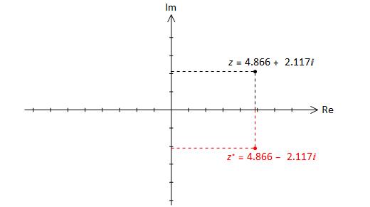
Fig. 3.1 Representation of a complex number in the complex plane (also known as an Argand diagram). The real part of the number is represented on the horizontal axis, and the imaginary part is represented on the vertical axis. \(z^*\) is given by reflecting the point z through a mirror placed along the real axis (negating the imaginary part).

3.2.2. The modulus and argument of a complex number

The representation \(z=x+yi\) is known as the Cartesian form of a complex number. In graphical terms it tells us where the number lies with respect to the real and imaginary axes.

An alternative way of describing the location of a complex number in the plane is by proving the following two pieces of information:

Definition

The modulus or absolute value of \(z\), denoted by \(|z|\) or \(\mathrm{abs}(z)\), measures the length of the line connecting the point to the origin. It is always a positive quantity.

By inspecting Figure Fig. 3.2, we can see that the modulus is just the length of the hypothenuse of a right-angled triangle. The base and height of the triangle are given by the real and imaginary parts, and so we have

(3.3)\[|x+iy| = \sqrt{x^2+y^2}.\]

Definition

The argument of a complex number, denoted by \(\mathrm{arg}(z)\), measures the angle between the positive real axis and the line connecting the point to the origin. You might think of it as a bearing, relative to the direction of the positive real axis.

We measure the argument continuously in the anti-clockwise direction, and there are two different conventions in use for giving the argument of a complex number that lies below the real axis.

The two conventions are both illustrated in Fig. 3.2.

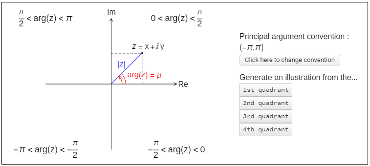
Fig. 3.2 Generic illustration of a complex number in the plane. The length of the blue line connecting the point to the origin is given by \(|z|=\sqrt{x_2+y_2}\). The angle subtended on the real axis is given by \(\mu=\mathrm{arctan}(|y/x|)\). There are two different conventions in use for measuring the argument. Click on the interactive figure to explore them both.

Attention

1. You must work in radians when providing the argument of a complex number. We will see later that there are special mathematical relationships involving the argument of a complex number, that are only valid when working in radians.

2. We will always give the argument in the range \([−\pi,\pi]\). This convention is much more common in the literature and also used by most mathematical computer software. Notice that conjugation in polar form is neater with this convention, since \(\mathrm{arg}(z^∗)=−\mathrm{arg}(z)\).

3. Strictly speaking, the argument as defined here is called the principal argument, since we could also locate the complex number by wrapping multiple times around the plane. For example, the argument \(−\pi/4\) could equally be given as \((2n−1/4)\pi\) for any integer value of \(n\).

3.3. Polar Form of a Complex Number

The relationship between the Cartesian representation \(z = x + yi\) and the modulus & argument representation is illustrated in Fig. 3.2. We conclude that a complex number can be expressed in the form:

(3.4)\[z = r(\cos(\theta) + i \sin(\theta)).\]

An alternative way of writing this result is the celebrated polar form of a complex number, using the exponential function:

(3.5)\[z = re^{i\theta} = r(\cos(\theta) + i \sin(\theta)), \textrm{where } r = |z|, \theta = \arg(z)\]

We will understand (and prove!) this result later. For now, we just find the polar representation of given complex numbers, and use the polar form to deduce some further results.

Practice Questions

Note: It is usually best to draw a diagram showing the location of the complex numbers in the plane, especially when just starting out. This will help avoid mistakes!

1. Write down the polar form of the following complex numbers:

a. \(1+i\)

b. \(-1+i\)

c. \(-1-i\)

d. \(1-i\)

e. \(-1\)

2. Express the following complex numbers in Cartesian form:

a. \(\sqrt{3}e^{-i\pi /3}\)

b. \(e^{i\pi /2}\)

Solution

1. All of the problems in 1(a)-1(d) have a modulus of \(\sqrt{2}\) and subtend an angle of \(\frac{\pi}{4}\) with the real axis. Thus, we have:

a. \(1+i \equiv \sqrt{2}e^{\frac{i\pi}{4}}\)

b. \(-1+i \equiv \sqrt{2}e^{\frac{3i\pi}{4}}\)

c. \(-1-i \equiv \sqrt{2}e^{\frac{-3i\pi}{4}}\)

d. \(1-i \equiv \sqrt{2}e^{\frac{-i\pi}{4}}\)

e. Since \(-1\) lies on the negative real axis, it has an argument of \(\pi\) and modulus \(1\), so \(e^{i\pi} = -1\) and hence, we can write the famous result \(e^{i\pi} + 1 = 0\).

2. Using the result that \(e^{i\theta} = \cos(\theta) + i\sin(\theta)\) gives:

a. \(\sqrt{3}e^{-i\frac{\pi}{3}} = \sqrt{3}(\cos(\frac{\pi}{3} - i\sin(\frac{\pi}{3})) = \sqrt{3}(\frac{1}{2} - i\frac{\sqrt3}{2}) = \frac{\sqrt3}{2} - i\frac{3}{2}\)

b. \(e^{i\frac{\pi}{2}} = i\)

Both results could also be derived by sketching the numbers in the plane.

3.4. Complex Arithmetic

3.4.1. Addition and Subtraction

To add or subtract complex numbers, we simply add or subtract the real and imaginary parts:

(3.6)\[(x_1+y_1i) \pm (x_2+y_2i) = (x_1 \pm x_2) + (y_1 \pm y_2)i\]

We can represent the result of the addition graphically by constructing a parallelogram from the three complex points

• \(z_1 = x_1 + y_1i\),

• \(z_2 = x_2 + y_2i\),

• \(z_3 = z_1 + z_2\)

as shown in Fig. 3.3.

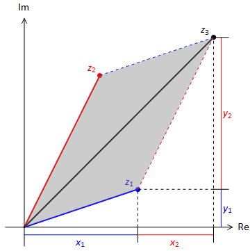
Fig. 3.3 Parallelogram rule for addition of complex numbers, \(z_3 = z_1+z_2\)

A graphical representation of the result for subtraction is shown in Fig. 3.4. notice that \(z_3 = z_2-z_1\) rearranges to give \(z_2 = z_1-z_3\), so now \(z_2\) is lies on the diagonal of the parallelogram.

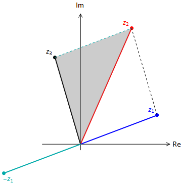
Fig. 3.4 Triangle rule for subtraction of two complex numbers, \(z_3=z_2-z_1\).

3.4.2. Multiplication of complex numbers

The product of two complex numbers is just an ordinary product of sums, and so follows the FOIL rule (Firsts, Outsides, Insides, Lasts):

(3.7)\[\begin{split}(x_1+y_1i)(x_2+y_2i) &= x_1x_2 + ix_1y_2 + ix_2y_1 + i^2y_1y_2 \\ &= (x_1x_2 - y_1y_2) + i(x_1y_2 + x_2y_1)\end{split}\]

Note the use of \(i^2=-1\) to simplify the result.

Practice Questions

1. Let \(z=1+2i\), and \(w=2-i\). Calculate \(z\,w^*\).

2. Show that the result \(zz^* = |z|^2\) is true for any complex number z. (This result is useful, and should be remembered.)

Solutions

1. \(z\,w^* = (1+2i)(2-i) = 2-i+4i+2 = 3+3i\)

2. Let \(z=x+yi\),

then \(zz^* = (x+yi)(x-yi) = x^2 + yi - yi + i^2y = x^2 + y^2 = |z|^2\)

3.4.3. Division of Complex Numbers

Suppose that \(z_1 = x_1 + iy_1\), \(z_2 = x_2 + iy_2\) and we want to express the result \(z_3 = \frac{z_1}{z_2}\) in the form \(z_3 = x_3 + iy_3\) where \(x_3\) and \(y_3\) are real numbers.

We make use of the fact that \(zz^*\) is real to make sure we get a real number in the denominator of the resulting fraction:

(3.8)\[z_3 = \frac{z_1}{z_2}\frac{z_2*}{z_2*} = \frac{z_1z_2*}{|z_2|^2}\]

Here we have just multiplied by \(1\), as \(\frac{z_2*}{z_2*} = 1\).

Let’s see how this works for an example in which \(z_1 = 2 + 3i\) and \(z_2 = 1 - 2i\):

(3.9)\[\frac{2+3i}{1-2i} = \frac{2+3i}{1-2i} \frac{1+2i}{1+2i} = \frac{2+3i+4i-6}{1+4} = -\frac{4}{5} + \frac{7}{5}i\]

Practice Questions

1. Simplify the expression :

\[\frac{7+i}{1+3i}\]

2. Write the following expression in the form of \(z = x + iy\, x,\,y\in \mathcal{R}\):

\[z = \frac{1}{1-3i} + \frac{1}{1+3i} + 1+3i\]

Solution

1.

\[\frac{7+i}{1+3i} = \frac{7+i}{1+3i}\frac{1-3i}{1-3i} = \frac{7-21i+i+3}{1+9} = 1-2i\]

2.

\[\frac{1}{1-3i} + \frac{1}{1+3i} = \frac{1+3i}{1+3^2} + \frac{1-3i}{1+3^2} = \frac{2}{10} = \frac{1}{5}\]

and hence:

\[z = \frac{1}{5} + 1 + 3i = \frac{6}{5} + 3i\]

3.4.4. Multiplying and Dividing Complex Numbers in Polar Form

Multiplying and dividing complex numbers in polar form is particularly easy. If we suppose that \(z_1 = r_1e^{i\theta_1}\), and \(z_2 = r_2e^{i\theta_2}\), then the result follows immediately from the laws of exponents:

(3.10)\[z_1 z_2 = r_1 r_2 e^{i(\theta_1 + \theta_2)} = \frac{r_1}{r_2} e^{i(\theta_1 - \theta_2)}\]

These results highlight very clearly the geometry of multiplication and division in the complex plane. Notice in particular that multiplication by \(e^{i\theta}\) just rotates a complex number in the plane by and angle \(\theta\). What result would multiplication by \(e^{2\pi i}\) give?

The geometry of multiplication and division of complex numbers

• \(|z_1z_2| = |z_1||z_2|\)

• \(\textrm{arg}(z_1z_2) = \textrm{arg}(z_1) + \textrm{arg}(z_2)\)

When \(z_1\) is multiplied by \(z_2\):

• The distance of \(z_1z_2\) to the origin is increased by a factor of \(|z_2|\),

• The position of \(z_1z_2\) is rotated counter clockwise by an angle \(\textrm{arg}(z_2)\) relative to \(z_1\).

• \(|z_1/z_2| = |z_1|/|z_2|\)

• \(\textrm{arg}(z_1/z_2) = \textrm{arg}(z_1) - \textrm{arg}(z_2)\)

When \(z_1\) is multiplied by \(z_2\):

• The distance of \(z_1z_2\) to the origin is reduced by a factor of \(|z_2|\),

• The position of \(z_1z_2\) is rotated clockwise by an angle \(\textrm{arg}(z_2)\) relative to \(z_1\).

A good way to remember these rules is that in polar form, you can multiply two complex numbers by multiplying the magnitude and adding the angles.

Conversely, to divide two numbers in polar form, you divide the magnitude, and subtract the angles.

Practice Questions

1. For each of the following pairs of numbers, state the results \(|zw|\) and \(\textrm{arg}(zw)\), taking care to ensure that you give the argument in the principal domain.

a. \(z = -1+i\), \(w=\sqrt{3}+i\),

b. \(z = -1+i\), \(w = -\sqrt{3} + i\).

2. By writing \(z_1 = r_1e^{i\theta_1}\), \(z_2 = r_2e^{i\theta_2}\), prove the result:

\[\Big(\frac{z_1}{z_2}\Big)^* = \frac{z_1^*}{z_2^*}\]

Solution

1.

a. \(|z| = \sqrt{2}\), \(|w| = 2\), so \(|zw| = 2\sqrt{2}\) \(\textrm{arg}(z) + \textrm{arg}(w) = \frac{3}{4}\pi + \frac{\pi}{6} = \frac{11}{12}\pi = \textrm{arg}(zw)\)

b. \(|zw| = 2\sqrt{2}\) \(\textrm{arg}(z) + \textrm{arg}(w) = \frac{3}{4}\pi + \frac{5}{6}\pi = \frac{19}{12}\pi\), which lies in the fourth quadrant. The principal argument is given by \(\textrm{arg}(zw) = -\frac{5}{12}\pi\).

2.

\[\left(\frac{z_1}{z_2}\right)^* = \left(\frac{r_1e^{i\theta_1}}{r_2e^{i\theta_2}}\right)^* = \frac{r_1}{r_2} e^{-i(\theta_1 - \theta_2)} = \frac{r_1 e^{-i\theta_1}}{r_2 e^{-i\theta_2}} = \frac{z_1^* }{z_2^* }\]

3.5. Complex Roots

3.5.1. Periodicity of \(e^{i\theta}\)

Earlier we deduced that multiplication by \(e^{i\theta}\) corresponds to a rotation of a complex number by an angle \(\theta\).

For the special case of a complete rotation, \(\theta = 2\pi\), multiplication returns the complex number to its original location in the plane, and so we have the result \(e^{2\pi i} = 1\). In a general form, \(e^{2k\pi i} = 1\) for any whole number of rotations \(k\), with the sign of the exponent determining the direction of rotation.

Another way of viewing this result is in terms of the periodicity of the complex exponential. Euler’s formula tells us that the complex exponential \(e^{i\theta}\) is the linear sum of two \(2\pi\)-periodic functions, and so we can deduce that it also has a period of \(2\pi\). That is:

(3.11)\[e^{i(\theta + 2k\pi)} = e^{i\theta} \textrm{ for } k = 0, \pm1, \pm2, ...\]

Geometrically, the expression is merely a statement of the fact that if we continuously “wrap around” the complex plane without changing the modulus, we will return to our starting position at the end of each complete revolution.

This was also the principal by which we were able to define (at least) two different possible conventions for the principal argument.

Practice Questions

Write the following complex numbers in polar form where the argument is given in the principal range (\(-\pi\), \(\pi\)):

1. \(\sqrt{2}e^{\frac{7\pi i}{3}}\)

2. \(3e^{-\frac{13\pi i}{12}}\)

Solution

1. \(\frac{7\pi}{3} = 2\pi + \frac{\pi}{3}\) so the result lies in the first quadrant at an angle of \(\frac{\pi}{3}\) away from the real axis. The result can be written as \(\sqrt{2}e^{\frac{\pi i}{3}}\).

2. \(-\frac{13\pi}{12}\) lies in the second quadrant at an angle of \(\frac{\pi}{12}\) away from the real axis, so the equivalent to an argument of \(\pi - \frac{\pi}{12}\). The result can be written as \(3e^\frac{11\pi}{12}\).

3.5.2. Roots of Unity

In this subsection, we will deduce the roots of the problem \(z^m = 1\), where \(m\) is a natural number {1, 2, 3, …}. We call these results the \(m^{th}\) “roots of unity”.

From the basic laws of exponents, we can observe that taking:

(3.12)\[z_k = e^{i\frac{2k\pi}{m}}\]

gives \((z_k)^m = e^{2k\pi i}\), and these values are both equal to 1 if k is an integer.

Since the number of integers in infinite, it appears that we have found an infinite number of \(m^{th}\) roots of unity. However, we know that a degree \(m\) polynomial should have only \(m\) roots, which may not be distinct from one another, as all such polynomials can be obtained by multiplying together a product of \(m\) factors of the form \((z-z_k)\).

We can reconcile this apparent contradiction by again considering the periodicity of the complex exponential. You may verify that for the expression \(z_k\) given above, \(z_{k+m}=z_k\). and this means that after a run of \(m\) consecutive values of \(k\) the results will start to repeat.

Fig. 3.5 illustrates how the values of \(k\) can be chosen to give the roots in polar form where the argument is in the range (\(-\pi, \pi\)). The geometric location of the roots in the complex plane is also shown, illustrating the equal angular separation between the roots.

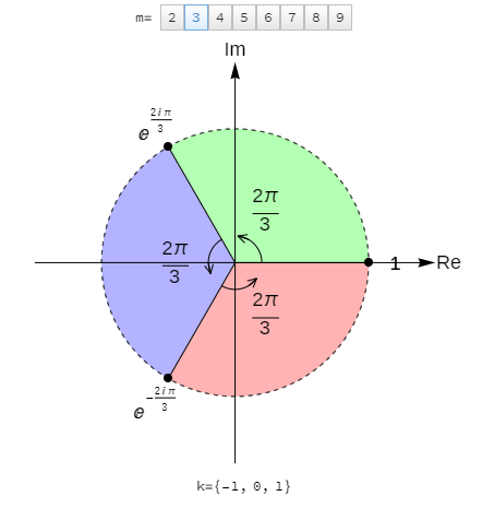
Fig. 3.5 An illustration showing the location of the roots of \(z^m=1\), which are of the form \(z=e^{\frac{2k\pi i}{m}}\).

Practice Questions

1. Have a go at finding all the roots of the problem \(z^3=1\) in Cartesian form.

Solution

1. The 3 roots of unity can be found at \(z=e^{i\frac{2n\pi}{3}}\) for \(n \in {0,1,2}\) and so the roots are

\[z = 1, \quad -\frac{1}{2}+\frac{\sqrt{3}}{2}i, \quad -\frac{1}{2}-\frac{\sqrt{3}}{2}i\]

3.5.3. Roots of Other Values

Now that we have solved the roots of unity, finding the complex roots of other values \(z^m = c\) is relatively straightforward, even in cases where \(c\) is complex value.

We simply express \(c\) in polar form, \(c=re^{i\theta}\), and then use the result:

(3.13)\[z_m = r^{1/m}e^{i \theta/m}e^{i 2\pi k/m},\, k \in \mathbb{Z}\]

Worked Example

Find all roots of the problem \(z^4 = \sqrt{3} - i\) in Cartesian form, \(z = x + iy\).

We begin by writing the right hand side in polar form: \(\sqrt{3} - i = 2e^{-i\pi/6}\)

Here, \(m=4\), and so we use Equation (3.13) to find our roots:

\[z_m = 2^{1/4}\,e^{i(-\pi/6 + 2\pi k)/3},\, k \in \mathbb{Z}\]

One solution is given simply by \(z_0 = (2e^{-i\pi/6})^{1/4} = 2^{1/4}e^{-i\pi/24}\)

Following through different values of \(m\), we obtain:

\[\begin{split}z_{-1} &= 2^{1/4}e^{-i 13\pi/24} \\ z_0 &= 2^{1/4}e^{-i \pi/24} \\ z_1 &= 2^{1/4}e^{i 11\pi/24} \\ z_2 &= 2^{1/4}e^{i 23\pi/24} \end{split}\]

We see that the other roots are found by multiplying by \(e^{-i\pi/2},\, e^{i\pi/2},\ e^{i\pi}\)

3.5.4. Polynomial roots

We can treat complex roots to polynomial just like any other real roots, which for an \(n^{th}\) order polynomial we can write as:

\[f(z) = az^n + bz^{n-1} + \dots =(z-z_1)(z-z_2)\dots(z-z_n) = 0\]

where here \(z_n \in \mathbb{C}\) in general.

We find by the conjugate root theorem, i.e. that if \(z_n\) is a complex root of \(f(z)\) then \({z_n}^*\) is also a root - this is not true in general if \(z_n\) is a real root.
It also follows from this that if \(n\) is odd, then the polynomial must have at least one real root.

Practice questions

1. The polynomial \(z^3 - 7z^2 + 41z - 87\) has a root \(z = 2 + 5i\), find all the other roots.

2. Find all the roots of \(z^4 - z^3 - z^2 - z - 2\), given that they are all integer points in the complex plane.

Solutions

1. If \(z_1 = 2 + 5i\), then \(z_2 = {z_1}^* = 2 - 5i\), hence we can factorise this polynomial as:

\[(z - 2 - 5i)(z - 2 + 5i)(z-a) = 0\]

where \(a\) here must be a real root. Expanding this out, we find:

\[(z^2 - 4z + 29)(z-a) = z^3 - (a + 4)z^2 + 25z - 29a = 0\]

which suggests that \(a=3\), hence the three roots are:

\[z = 3,\, 2+5i,\, 2-5i\]

2. If \(z^4 - z^3 - z^2 - z - 2\), we can spot that \(z = 2\) is a root, hence:

\[z^4 - z^3 - z^2 - z - 2 = (z-2)(z^3 + z^2 + z + 1) = 0\]

we can then spot that \(z = -1\) is also a root:

\[(z-2)(z^3 + z^2 + z + 1) = (z-2)(z+1)(z^2 + 1) = 0\]

and given that \(z^2 + 1 = (z-i)(z+i)\), we have our final two roots:

\[z^4 - z^3 - z^2 - z - 2 = (z-2)(z+1)(z + i)(z-i)\]

3.6. Trigonometric and hyperbolic relationships

In this section, we make use of Euler’s identity, \(e^{i\theta} \equiv \cos(\theta) + i\sin(\theta)\), to prove several results involving trigonometric and hyperbolic functions.

3.6.1. de Moivre’s theorem

Starting with Euler’s Identity \(e^{i\theta} \equiv \cos(\theta) + i\sin(\theta)\) and raising both sides to the \(n^{th}\) power gives:

(3.14)\[e^{in\theta} = (\cos(\theta) + i\sin(\theta))^n\]

We can then use Euler’s identity again (replacing \(\theta\) with \(n\theta\)) to re-write the left had side:

(3.15)\[\cos(n\theta) + i\sin(n\theta) \equiv (\cos(\theta) + i\sin(\theta))^n\]

This result (for integer values of \(n\)) is known as de Moivre’s theorem.

Non-integer Values

For non-integer values \((\cos(\theta) + i\sin(\theta))^n\) is multiple-valued. The principal root is normally taken as the one that has the smallest positive argument, or that gives a real number. The result \(\cos(n\theta) + i\sin(n\theta)\) gives a single root to the problem, but not necessarily the principal root.

3.6.2. Compound angle formulae

The derivation of trigonometric identities is tremendously simplified using complex exponentials. For example:

(3.16)\[\begin{split}e^{i(A+B)} &= e^{iA}e^{iB}\\ \cos(A+B) + i\sin(A+B) &= (\cos(A) + i\sin(A))(\cos(B) + i\sin(B))\end{split}\]

Expanding out the right hand side and comparing the real and imaginary parts provides us with the compound angle formula for \(\cos(A+B)\) and \(\sin(A+B)\). We obtain the familiar results:

(3.17)\[\begin{split}\cos(A+B) &= \cos(A)\cos(B) - \sin(A)\sin(B) \\ \sin(A+B) &= \sin(A)\cos(B) + \cos(A)\sin(B)\end{split}\]

In some applications (e.g. integration), we will occasionally need to express trigonometric powers in terms of multiple angles , a common one being \(\cos^2(\theta) = \frac{1}{2}(\cos(2\theta)+1)\).

For higher powers we make use of the complex exponential form:

\[\begin{split}\cos(\theta) &= \frac{1}{2}\Big(e^{i\theta} + e^{-i\theta} \Big) \\ \sin(\theta) &= \frac{1}{2i}\Big(e^{i\theta} - e^{-i\theta} \Big) \end{split}\]

and therefore:

\[\begin{split}\cos^n(\theta) &= \frac{1}{2^n}\Big(e^{i \theta} + e^{-i\theta} \Big)^n \\ &= \frac{1}{2^n}\Big(e^{ni\theta} + e^{-ni\theta} + ne^{(n-2)i\theta} + ne^{-(n-2)i\theta} + \dots \Big)\\ &= \frac{1}{2^{n-1}}\Big(\cos(n\theta) + n\cos((n-2)\theta) + \dots \Big)\\ \sin^n(\theta) &= \frac{1}{(2i)^n}\Big(e^{i \theta} - e^{-i\theta} \Big)^n \\ &= \frac{1}{(2i)^n}\Big(e^{ni\theta} - e^{-ni\theta} + ne^{(n-2)i\theta} - ne^{-(n-2)i\theta} + \dots \Big)\\ &= \frac{1}{(2i)^{n-1}}\Big(\sin(n\theta) + n\sin((n-2)\theta) + \dots \Big)\end{split}\]

where we can expand out using binomial theorem. We note that for \(n\) odd that will be \((n+1)/2\) trigonometic terms in the expansion and for \(n\) even there will be \(n/2\) trigonometric terms in the expansion as well as a constant term.

Practice Questions

1. Show that:

\[\cos^7(\theta) = \frac{1}{64} \Big[35\cos(\theta) + 21\cos(3\theta) + 7\cos(5\theta) + \cos(7\theta)\Big]\]

2. Find an expressions for \(\cos(7 \theta),\, \sin(7\theta)\) in terms of \(\cos(\theta),\, \sin(\theta)\).

3. Find an expression for \(\sin^5(\theta)\) in terms of \(\sin(n\theta),\, n \in \mathbb{N}\).

Solutions

1. Given that \(\cos(\theta) = \frac{1}{2}\Big(e^{i \theta} + e^{-i \theta}\Big)\), then we can find \(\cos^7(\theta)\) as:

\[\begin{split}\cos^7(\theta) &= \Big[\frac{1}{2}\Big(e^{i \theta} + e^{-i \theta}\Big)\Big]^7 \\ &= \frac{1}{2^7}\Big( e^{7 i \theta} + 7e^{6 i \theta}\,e^{-i \theta} + 21e^{5 i \theta}\,e^{-2i \theta} + 35e^{4 i \theta}\,e^{-3i \theta} + 35e^{3 i \theta}\,e^{-4i \theta} + 21e^{2i \theta}\,e^{-5i \theta} + 7e^{i \theta}\,e^{-6i \theta} + e^{-7i \theta} \Big)\\ &= \frac{1}{2^7}\Big( e^{7 i \theta} + e^{-7i \theta} + 7e^{6 i \theta}\,e^{-i \theta} + 7e^{i \theta}\,e^{-6i \theta} + 21e^{5 i \theta}\,e^{-2i \theta} + 21e^{2i \theta}\,e^{-5i \theta} + 35e^{4 i \theta}\,e^{-3i \theta} + 35e^{3 i \theta}\,e^{-4i \theta} \Big)\\ &= \frac{1}{2^7}\Big( e^{7 i \theta} + e^{-7i \theta} + 7\,e^{5i \theta} + 7\,e^{-5i \theta} + 21z,e^{3 i \theta} + 21\,e^{-3i \theta} + 35e^\,e^{-i \theta} + 35\,e^{-i \theta} \Big)\\ &= \frac{1}{128}\Big[2\cos(7 \theta) + 7(2\cos(5 \theta)) + 21(2\cos(3 \theta)) + 35(2\cos(\theta))\Big]\\ \Rightarrow \cos^7(\theta)&= \frac{1}{64}\Big[\cos(7 \theta) + 7\cos(5 \theta) + 21\cos(3 \theta) + 35\cos(\theta)\Big]\\\end{split}\]

2. Starting with:

\[\Big(e^{i\theta}\Big)^7 = \Big(\cos(\theta) + i \sin(\theta)\Big)^7 = e^{7i\theta}= \cos(7\theta) + i \sin(7\theta)\]

then by expanding out the terms in the binomial and collecting the real and imaginary parts we find:

\[\begin{split}\Big(\cos(\theta) + i \sin(\theta)\Big)^7 &= \cos^7(\theta) + 7i \cos^6(\theta)\,\sin(\theta) - 21 \cos^5(\theta)\,\sin^2(\theta) \\ & - 35i \cos^4(\theta)\,\sin^3(\theta) + 35 \cos^3(\theta)\,\sin^4(\theta) \\ &+ 21i \cos^2(\theta)\,\sin^5(\theta) - 7 \cos(\theta)\,\sin^6(\theta) - i \sin^7(\theta) \end{split}\]

and hence:

\[\begin{split}\cos(7\theta) &= \cos^7(\theta) - 21 \cos^5(\theta)\,\sin^2(\theta) + 35 \cos^3(\theta)\,\sin^4(\theta) 7 \cos(\theta)\,\sin^6(\theta) \\ \sin(7\theta) &= 7 \cos^6(\theta)\,\sin(\theta) - 35 \cos^4(\theta)\,\sin^3(\theta) + 21 \cos^2(\theta)\,\sin^5(\theta) - \sin^7(\theta) \end{split}\]

3. Given that:

\[\sin^5(\theta) = \Big(\frac{1}{2i}\Big)^5\Big(e^{i\theta}-e^{-i\theta}\Big)^5\]

Expanding out the right hand side using binomial expansion, and collecting together powers of \(\theta\) gives:

\[\begin{split}\sin^5(\theta) &= \left(\frac{1}{2}\right)^5 (-i) [(e^{5i\theta} - e^{-5i\theta}) - 5(e^{3i\theta} - e^{-3i\theta}) + 10(e^{i\theta} - e^{-i\theta})]\\ &= \left(\frac{1}{2}\right)^5 (-i) [2i\sin(5\theta) - 5(2i)\sin(3\theta) + 10(2i)\sin(\theta)]\\ &= \frac{1}{16} [\sin(5\theta) - 5\sin(3\theta) + 10\sin(\theta)]\\ \end{split}\]

3.6.3. Hyperbolic functions

Hyperbolic functions can be thought of as a way to take the exponential function \(e^{x}\) which is neither odd nor even and generate odd or even functions from it. To do so, think about the graphs of \(e^{x},\, e^{-x}\) which are mirror images in the \(y\) axis:

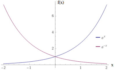
Fig. 3.6 Graphs of \(e^{x},\, e^{-x}\).

If we add up these functions, \(e^{x} + e^{-x}\), we find a function which looks like:

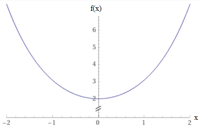
Fig. 3.7 Graph of \(e^{x}+e^{-x}\).

which clearly now has the property that \(f(-x) = f(x)\), i.e. it is even. Likewise if we subtract one function from another \(e^{x} - e^{-x}\), it looks like:

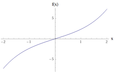
Fig. 3.8 Graph of \(e^{x}-e^{-x}\).

and again this now has the property that \(f(-x) = -f(x)\), i.e. is is odd.

Therefore from a function that is neither, we can construct odd and even functions, by convention we will halve the resultign functions so that \(\cosh(\theta)\) has a minima of unity at the \(y\) axis.

Defintions of hyperbolic functions

\[\begin{split}\cosh(\theta) &= \frac{1}{2}\Big(e^{x} + e^{-x} \Big) \\ \sinh(\theta) &= \frac{1}{2}\Big(e^{x} - e^{-x} \Big)\end{split}\]

We can then also define the hyperbolic tangent \(\tanh(\theta)\) as:

\[\tanh(\theta) = \frac{\sinh(\theta)}{\cosh(\theta)} = \frac{e^{x} + e^{-x}}{e^{x} - e^{-x}} = \frac{e^{2x}+1}{e^{2x}-1}\]

and finally, essentially define a hyperbolic form of any trigonometric function:

\[\begin{split}\textrm{sech} &= \frac{1}{\cosh(\theta)} = \frac{2}{e^x + e^{-x}} = \frac{2e^x}{e^{2x} + 1} \\ \textrm{cosech}(\theta) &= \frac{1}{\sinh(\theta)} = \frac{2}{e^x - e^{-x}} = \frac{2e^x}{e^{2x} - 1} \\ \coth(\theta) &= \frac{1}{\tanh(\theta)} = \frac{e^{x} - e^{-x}}{e^{x} + e^{-x}}= \frac{e^{2x}-1}{e^{2x}+1}\end{split}\]

Practice questions

1. Find real solutions to the problem \(\cosh(x) = 2\)

2. Find all the real solutions to the problem:

\[2 \sinh(x) = \cosh(x)\]

Solutions

1.

\[\cosh(x) = \frac{1}{2}\Big(e^x + e^{-x} \Big) = 2\]

which is a disguised quadratic in \(e^x\):

\[e^{2x} + 1 = 4e^{x} \Rightarrow e^{2x} - 4e^{x} + 1 = 0\]

which has roots of:

\[e^{x} = 2 \pm \sqrt{3} \Rightarrow x_\pm = \ln \Big( 2 \pm \sqrt{3}\Big)\]

2.

\[2\Big(e^{x} - e^{-x}\Big) = e^{x} + e^{-x}\]

which is a disguised quadratic in \(e^x\):

\[\begin{split}2\Big(e^{2x} - 1\Big) &= e^{2x} + 1 \\ e^{2x} &= 3 \\ x &= \frac{1}{2}\ln(3)\end{split}\]

3.6.4. Relationship between trigonometric and hyperbolic functions

Starting from Euler’s identity, we observe that:

(3.18)\[\begin{split}e^{i\theta} &= \cos(\theta) + i\sin(\theta) \\ e^{-i\theta} &= \cos(\theta) - i\sin(\theta)\end{split}\]

By adding and subtracting these two results, we obtain expressions for cosine and sine in terms of complex exponentials, which are strikingly similar to the hyperbolic cosine and sine functions:

(3.19)\[\begin{split}\cos(\theta) = \frac{1}{2}(e^{i\theta}+e^{-i\theta}) &= \cosh(i\theta)\\ \sin(\theta) = \frac{1}{2i}(e^{i\theta}-e^{-i\theta}) &= -i\sinh(i\theta)\end{split}\]

and likewise if we redefine \(\theta = ix\):

\[\begin{split}\cosh(x) & = \cos(ix) \\ \sinh(x) &= -i\sin(ix)\end{split}\]

The results may be used to obtain similar results for functions like \(\tan(\theta)\) etc:

\[\tan(\theta) = \frac{\sin(\theta)}{\cos(\theta)} = \frac{-i\sinh(i\theta)}{\cosh(i\theta)} = -i\tanh(i\theta)\]

3.6.5. Compound hyperbolic identities

We can see from the relationships between trigonometric and hyperbolic functions in (3.19) that if we raise trignomietric functions to power (e.g. squaring them), there are related hyperbolic identities:

\[\begin{split}\cos^2(\theta) &= \cosh^2(i \theta) \\ \sin^2(\theta) &= -\sinh^2(i \theta)\end{split}\]

therefore trigonmetric identities can be modified to become hyperbolic identities:

\[\begin{split}\cos^2 (\theta) + \sin^2(\theta) = 1 &\Longleftrightarrow \cosh^2(x) - \sinh^2(x) = 1\\ \sin(2\theta) = 2\sin(\theta)\,\cos(\theta) &\Longleftrightarrow \sinh(2\theta) = 2\sinh(\theta)\,\cosh(\theta) \\ \cos(2\theta) = \cos^2(\theta) - \sin^2(\theta) &\Longleftrightarrow \cosh(2\theta) = \cosh^2(\theta) + \sinh^2(\theta) \end{split}\]

previous

2. Binomial Expansion and Theorem

next

4. Limits of Functions and Sequences