Sequences and Series
Contents
5. Sequences and Series
5.1. Sequences
Definition
A sequence is a set of terms where order matters, written as follows:
Here, the size of the sequence (the number of terms) is \(n\). The \(i\)-th term in the sequence may be denoted by \(u_i\) where \(i = 1, 2, \dots, n\).
The labels \(u\), and \(i\) are arbitrary, and we could just as well use other letters to represent them. Sequences can have finite \(n<\infty\) (e.g. telephone numbers) or infinite sizes \(n \to \infty\) (e.g. the prime numbers).
The sequences that we will examine in this course are numerical patterns. Much of mathematics is concerned with patterns in both mathematical constructs and nature, and the study of sequences provides a firm grounding for this endeavour.
Mathematical patterns can generally be expressed as formula for the \(i\)th term. For instance, the formula below generates the sequence \(-1, 2, 5, 8, 11, 14, 17, 20\) by taking \(i=1,\dots 8\) :
Notice that the size of the terms in this sequence grows without bound as the number of terms is increased.
5.1.1. Recurrence relationships
It is sometimes possible to express a sequence as a formula that relates the \(n\)th term of the sequence as some combination of the previous terms. This is known as a recurrence relation.
Definition
A well-know example that arises in many natural systems is the Fibonacci sequence:
This sequence is generated by starting with the sequence \(1,1\) and finding the next number in the sequence by adding the two previous numbers together, e.g. \(0+1=\mathbf{1}\), \(1+1=\mathbf{2}\), \(1+2=\mathbf{3}\), \(2+3=\mathbf{5}\), \(3+5=\mathbf{8}\), etc.
The sequence can be expressed with the recurrence relation
The recurrence relation (5.2) specifies the \(i\)-th term provided we have the term for \(i-1\) and \(i-2\). It is because of this formula that it is necessary to provide the first two terms of the sequence, \(u_1=0\) and \(u_2=1\), to find the rest of the sequence.
Python code for Fibonacci sequence
Note that the Fibonnaci recurrence relation will generate a different sequence to the Fibonacci sequence when the starting terms are different (e.g. \(u_1=10\) and \(u_2=11\)).
nterms = 10 # number of terms
u1, u2 = 1, 1 # first two values
count = 0 # counter
while count < nterms: # while loop
       print(u1) # print values
       nth = u1 + u2 # recurrence relation
       u1 = u2 # update values
       u2 = nth # update values
       count += 1 # update counter
1
1
2
3
5
8
13
21
34
55
Practice Question
What sort of numbers does the recurrence relation \(u_i = 2 + u_{i-1}\) produce when \(u_1=2\) and when \(u_1=1\)?
A sequence is defined by the recurrence relation \(u_{n+1} = 3u_{n}\) with \(u_1 = 1\), determine the formula for \(u_n\).
Solution
We can write a Python script to generate the recurrence relation \(u_i = 2 + u_{i-1}\):
nterms = 10 # number of terms
u = 1 # first value
count = 0 # counter
while count < nterms: # while loop
       print(u) # print values
       u = u + 2 # recurrence relation
       count += 1 # update counter
If we run the code, we will see that this recurrence relation produces odd numbers if \(u_1 = 1\) and even numbers if \(u_1 = 2\).
If we run the code, we will see that this recurrence relation produces \(u_n = 3^n\).
Recurrence relations, although simple, can produce surprisingly complicated behaviours. For further reading you may like to study the logistic map:
where \(r\) is a constant. This equation (which models amongst other things animal population growth) opened up the field of chaos theory.
5.2. Series
Series play a central role in calculus and are the main reason why we introduce sequences in the section above.
Definition
A series is the sum of a sequence of terms, written as follows:
where \(m \le n\), and usually \(m=1\).
In short, a series is simply the sum of a sequence. We can replace the upper value \(n\) with \(\infty\) for an [infinite series. To give an example, the series of the infinite sequence \((u_1,u_2,u_3,\dots)\) is written as \(\displaystyle\sum_{i=1}^\infty u_i\).
We say that \(\displaystyle\sum_{i=m}^n u_i\) for \(n < \infty\) is a partial sum because the series is partially added up to just the \(n\)-th term.
Python Code
Here is some Python code for a sequence defined by the recurrence relation \(u_k = u_{k-1}+\frac{1}{2}\) with \(u_1=0\). It calculates the first ten terms of the sequence and the resulting series.
n = 10 # number of terms
seq = 0 # first value of sequence
ser = 0 # first value of series
count = 0 # counter
while count < n: # while loop
       print(seq, ser) # print series value
       seq = seq + 0.5 # update sequence
       ser = ser + seq # update series
       count += 1 # update counter
0 0
0.5 0.5
1.0 1.5
1.5 3.0
2.0 5.0
2.5 7.5
3.0 10.5
3.5 14.0
4.0 18.0
4.5 22.5
5.2.1. Summations
Character \(\Sigma\) is the Greek letter sigma, written in upper case, and denotes a summation.
We would read \(\sum_{i=1}^n u_i\) as “the sum of \(u_i\) from \(i=1\) to \(i=n\)”.
For example
is the sum of \(i\) from \(i=1\) to \(i=4\)
is the sum of \(2 i\) from \(i=1\) to \(i=4\)
From this example it should be clear that, in general:
where \(a\) is a constant.
Warning!
Take note that
For example, \(\displaystyle \sum_{i=1}^4 (1+i) = 2 + 3 + 4 + 5 = 14\).
The correct way to read this is:
Practice Questions
Write the following expressions using as a sum (\(\Sigma\) notation) without evaluating the sum:
\(1 + 5 + 9 + 13 + 17 +21\)
\(64-32+16-8+4-2+1\)
\(\frac{1}{3} + \frac{1}{4} + \frac{1}{5} + \dots + \frac{1}{99} \)
Solutions
1. \(\displaystyle\sum_{i=1}^6 (4n - 3)\)
or equivalently \(\displaystyle\sum_{i=0}^5 (4n + 1)\).
2. \(\displaystyle\sum_{i=0}^6 (-1)^n 2^{6 - n}\)
or equivalently \(\displaystyle\sum_{i=0}^6 (-1)^n 2^n\), by reversing the order of the summation.
3. \(\displaystyle\sum_{i=3}^{99} \frac{1}{n}\)
or equivalently \(\displaystyle\sum_{i=1}^{97} \frac{1}{n+2}\).
other answers are also possible!
5.3. Arithmetic and geometric progressions
We now introduce the arithmetic progression (or the arithmetic sequence) and the geometric progression (or geometric sequence). These sequences have the nice property that their series can be found straightforwardly.
5.3.1. Arithmetic progression
Definition
An arithmetic progression (otherwise known as an arithmetic sequence) is a sequence of \(n\) terms which all have a “common difference” \(d\), written as follows:
where \(a\) is an arbitrary number.
An example of an arithmetic progression is the sequence \(3,5,7,9,11,13\) in which the first term is \(a=3\), the common difference is \(d=2\) and the number of terms is \(n=6\). An infinite arithmetic progression is given by the case where \(n \to \infty\).
The \(i\)-th term of the arithmetic progression can be expressed as the following recurrence relation:
Python code for arithmetic progression
You can play around with the behaviour of different arithmetic progressions by changing the values of \(a\) and \(d\):
n = 10 # number of terms
a = 30 # first value
d = -4 # commmon difference
seq = a # first value of sequence
count = 0 # counter
while count < n: # while loop
       print(seq) # print series value
       seq = seq + d # update sequence
       count += 1 # update counter
30
26
22
18
14
10
6
2
-2
-6
5.3.1.1. Solving the series of arithmetic progressions
Series of arithmetic progressions can be solved (i.e. reduced to a number). The series (or the sum) \(S_n\) of an arithmetic progression with recurrence relation \(u_i=a+(i-1)d\) is:
where \(L = a + (n-1) d\) is the last term in the series.
As \(n\) approaches \(\infty\), the arithmetic progession approaches \(\infty\) if \(d>0\) and approaches \(-\infty\) if \(d<0\). In these cases we say that the series diverges (more on this later!). Infinite arithmetic progressions always diverge, the proof of which can be found via this link (although further reading is required!).
Python code for the series of the arithmetic progression
You can use this code to convince yourself that the series of arithmetic progressions grow without bound for large \(n\). In this ecxample we pick \(a = 30\), \(d=-4\).
nterms = 10 # number of terms
a = 30 # first value
d = -4 # commmon difference
seq = a # first value of sequence
ser = a # first value of series
count = 0 # counter
while count < nterms: # while loop
       print(ser) # print series value
       seq = seq + d # update sequence
       ser = ser + seq # update series
       count += 1 # update counter
30
56
78
96
110
120
126
128
126
120
Proof of the solution of the series of arithmetic progressions
Adding these two expressions gives:
Since there are \(n\) terms, this equations simplifies to the final result:
There is a legend, that Gauss (a famous mathematician) used a similar approach as a schoolboy back in the 1780s to find the answer to \(1+2+\dots+99+100\).
Practice Questions
How many terms are in the sequence \(54, 52, 50,\dots, 18\)?
Find the sum of the first 30 terms of the arithmetic progression with the first three terms \(3,9,15\).
Find the sum of the arithmetic progression with first term 2, last term 10 and common difference 2.
Evaluate \(\sum_{n=1}^{10} (5n-1)\) and \(\sum_{n=100}^{1000} n\) .
In an arithmetic progression the 3rd term is 26 and the 8th term is 46. Find the 1st term, the common difference and \(S_{50}\).
Find the sum of the integers between 1 and 100 which are divisible by 6.
Solution
1. This is an arithmetic progression (AP) with first term \(a=54\), common difference \(d=-2\), and last term \(L=18\).
Since \(L = a + (n-1)d\), we have \(n = \frac{18-54}{-2} = 19\) terms.
2. For an AP with first term \(a=3\), and common difference \(d=6\), the sum of the first \(30\) terms is given by
3. For this AP the first term is \(a=2\), the common difference is \(d=2\).
The last term is given by \(a+(n-1)d=10\), so we find that \(n=5\).
The sum is given by \(S_5 = \frac{5}{2} (2+10) = 30\).
4. The first expression is an AP with first term \(a=4\), last term \(L=49\) and \(n=10\) terms.
The sum is \(\frac{n}{2}(a+L)=265\).
The second expression is an AP with first term \(n=100\), last term \(L=1000\) and \(n=901\) (take care!).
The sum is \(\frac{n}{2} (a+L) = 495550\).
You could also calculate this using \(\frac{1000}{2}(1+1000)−\frac{99}{2}(1+99)\).
5. Let the first term of this AP be denoted by \(a\), and the common difference be denoted by \(d\).
We have that \(a+2d=26\) and \(a+7d=46\). Solving these two equations simultaneously gives \(a=18\) and \(d=4\).
The sum of the first \(50\) terms is given by:
6. The series is given by \(S=6+12+18+...+96 = \sum_{n=1}^{16} 6 n\).
This is the sum of an AP with first term \(a=6\), last term \(L=96\) and \(n=16\) terms.
The result is \(S= \frac{16}{2}(6+96)=816\).
5.3.2. Geometric progression
Definition
A geometric progression (otherwise known as an geometric sequence) is a sequence of \(n\) terms which have “common ratio” \(r\), written as follows:
where \(a\) is an arbitrary number.
Using the notation for sequences in the previous section, the \(i\)-th term of the geometric progression is \(u_i=a r^{i-1}\) for \(i=1,2,\dots,n\). In other words, the next term in the geometric progression can be found by multiplying the previous term by the common ratio \(r\), given by the recurrence relation \(u_i = r u_{i-1}\) where \(u_1=a\). An example is the sequence \(24,−12,6,−3,1.5\) in which the first term is \(a=2\), the common ratio is \(r=−\frac{1}{2}\) and the number of terms is \(n=5\).
Python code for a geometric progression
We can use some python code to examine this geometric progression, start at \(a=24\) and \(r = -0.5\):
nterms = 10 # number of terms
a = 24 # first value
r = -0.5 # commmon difference
seq = a # first value of sequence
count = 0 # counter
while count < nterms: # while loop
       print(seq) # print series value
       seq = seq * r # update sequence
       count += 1 # update counter
24
-12.0
6.0
-3.0
1.5
-0.75
0.375
-0.1875
0.09375
-0.046875
5.3.3. Solving the series of geometric progessions
Like arithmetic progessions, the series of geometric progressions can be solved (i.e. reduced to a number). The series (or the sum) \(S_n\) of a geometric progression \(u_i=a r^{i-1}\) is:
Python code for the series of the geometric progression
We can use some python code to examine the series of a geometric progression, start at \(a=24\) and \(r = -0.5\):
nterms = 10 # number of terms
a = 24 # first value
r = -0.5 # commmon difference
seq = a # first value of sequence
ser = seq # first value of series
count = 0 # counter
while count < nterms: # while loop
       print(seq) # print series value
       seq = seq * r # update sequence
       ser = ser + seq # update sequence
       count += 1 # update counter
24
-12.0
6.0
-3.0
1.5
-0.75
0.375
-0.1875
0.09375
-0.046875
Proof for the definition of a geometric series
we multiply by \(r\):
Subtracting \(r S_n\) from \(S_n\) and cancelling the terms provides:
And then dividing both sides by \(1-r\):
QED
If we have to deal with infinite geometric series, we argue that as \(n \rightarrow \infty\), \(S_n\) can either blow up or approach a finite value, this will depending whether \(r\) is large or small, but how to we define these more mathematically here?
One way to see this is to think about the proof for a geometric series:
Subtracting \(r S_n\) from \(S_n\) and cancelling the terms here means that almost all the terms cancel (this is only really true if the terms being cancelled add up to something finite):
And then dividing both sides by \(1-r\):
Another perspective is to think about the real number line, any numbers that are in the range \(0 < x < 1\), which are raised to an integer power, will definitely stay within this range. The same is also true if we extend this range out to positive and negative 1, i.e. formally:
(if we take any positive real power, then at least the real part will remain within this range).
This means that small and large here are determined by:
if \(\lvert r \rvert < 1\) then \(S_n\) converges as \(n\to \infty\),
if \(\lvert r \rvert > 1\) then \(S_n\) diverges as \(n\to \infty\).
If \(|r|<1\) then \(|r^n|<1\) and in the limit of \(n \rightarrow \infty\), \(|r|^n \rightarrow 0\), this makes the sum of an infinite geometric series:
We will make this more explicit when we discuss limits and convergence.
Practice Questions
Find the sum of the first five terms in a geometric progression with first term 27 and common ratio is \(2/3\)?
Evaluate:
The first term of a geometric progression is \(8\) and the sum of the first three terms is 38.
Given this find the two possible values of the common ratio.
A geometric progression has first term \(27\) and common ratio of \(r=\frac{4}{3}\).
Find the least number of terms that the sequence can have if its sum exceeds \(550\).
By writing the recurring decimal \(0.123123123\dots\) as a geometric progression, show that it can be expressed as the fraction \(\frac{41}{333}\).
Solutions
1. \(a=27\), \(r=\frac{2}{3}\),
2. The given expression represents the sum of a geometric progression (GP) with first term \(a=729\) and common ratio \(r=\frac{1}{3}\).
The sum over all integers n is given by \(S_{\infty}=\frac{729}{1−1/3}=\frac{2187}{2}\).
3. Let the first term of this GP be denoted by \(a\) (\(=8\)), and the common ratio be denoted by \(r\).
We have the sum of the first 3 terms is \(8(1+r+r^2)=38\).
4. The sum of the first \(n\) terms in this GP is given by \(S_n= 27 \frac{1−(4/3)^n}{1−4/3}\).
We require that \(S_n>550\). The problem could be tackled by trial and error, but we will solve it analytically.
The problem rearranges to give \((\frac{4}{3})^n>\frac{631}{81}\) (take care with the direction of the inequality!).
By taking the natural logarithm we obtain
Since \(n\) is an integer, the least number of terms required is \(8\).
5. Recurring decimals can we written as a series of fracitions:
which we can read as a geometris series, with \(a = 123/1000\) and \(r = 1/1000\), which means that:
5.4. Partial fractions
Consider the problem of adding different fractions, for example:
the easiest way to write this as one single fraction is to rewrite each fraction in terms of a common denominator and then just add the numerators. To find the common denominator, we need to find the lowest common multiple (LCM) of the denominators, here LCM\((2,3) = 6\) and hence:
If we have two algebraic fractions, we can follow a similar process:
An algorithm for finding partial fractions
1. If the degree of the numerator \(m\) is greater than (or equal to) the degree of the denominator \(n\), split off the leading terms in the form of a polynomial of degree \(m-n\).
2. Split up the remaining fraction so that the degree of each numerator is one less than the degree of the denominator.
3. To find the unknown constants, combine the fractions on the right hand side and equate the coefficients in the numerators on the left and right.
Worked Examples
1.
first split this up into:
and then recombine to set up equations to find the unknown coefficients:
There are two (equally valid) methods to use at this point to find \(A,\, B\):
a. We can substitute in \(n=1, \,-2\) into the equation, in each case:
b. We can compare coefficients of \(n^0\) and \(n^1\) (which by the fundamental theorem of algebra are independent), producing a set of simultaneous equations:
If we have repeated roots in the denominator, the decomposition now has terms for each of the roots and an additional one for the repeated root.
2.
To find the partial fractions, recall we first combine:
and then substitute in values:
3. Lets try to decompose \(\displaystyle \frac{11x+3}{x^2 + 3x + 2}\) into partial fractions:
To obtain the required fraction, we need \((A+B)x+(2A+B)=11x+3\), which by comparing coefficients of \(x\) we find two simultaneous equations:
We can solve these by choosing \(A=-8,\ B=19\), hence the result is:
This technique allows us to easily integrate:
4. Consider the function:
It can be decomposed as follows:
This gives:
and by expanding out:
Equating coefficients on the left and right sides we obtain simultaneous equations:
which is solved by \(A = -2/3,\, B = 4/3,\, C = 2/3\). This means that:
However, we can decompose this fraction further by noting that \((x^2-1)=(x+1)(x-1)\), therefore the full decomposition is:
An Application with Prime Factors
For a fraction like \( \frac{1}{18}\), can we decompose this into fractions of the prime factors \( 18 = 2\cdot 3^2\) ? The full partial fraction decomposition would have the form:
First we have to present the system in a way that is meaningful to use partial fractions:
so that we reduce to the original problem at \(f(0)\). Now we just follow the process
Substituting in values we find:
giving the final decomposition:
Practice Questions
Decompose the following into partial fractions:
1.
2.
3.
4.
Solutions
1.
Therefore by equating numerators:
so we find:
2.
Which means that:
and therefore by equating numerators:
so we find:
3.
4.
and therefore by equating numerators:
which means that \(A = 1,\, B = 2\) and so:
5.5. Method of differences
The method of differences provides a way to find a finite series (sum of a sequence) by using the difference of similar sums to compute the desired result. This is a handy trick to find the value of partial (finite) sums .
5.5.1. Writing out the series method
Lets start with a simple example:
we can expand out this series term by term and see some cancellation occurs:
A question may appear not to have an obvious difference set out, such as:
For a fraction of this form however, we can make use of partial fractions:
Equating numerators gives:
and so looking again at the series:
which is now in the form of method of differences.
Expanding out the first few and last few terms allows us to spot the pattern:
If we have a series which is composed of an infinite number of terms, it is possible to apply the method of differences to see if it converges. An example:
which we can rewrite as:
and after solving by method of differences, take the limit \(N \rightarrow \infty\):
5.5.2. Rewriting the summation index method
It is possible to demonstrate the cancellation of terms without writing out the terms in the series.
In general, rewriting the summation index provides:
where \(f(r)\) is an arbitrary function of summation index \(r\) and \(c\) is a positive integer number.
This can be also used for negative integer values:
You will find that this technique can drastically simplify summations we wish to solve.
For example:
Practice Questions
Use the result \((r+1)^2 - (r-1)^2 = 4r\) to calculate \(\sum_{r = 1}^{N} r\) using both the writing out series and rewring the summation methods.
By using partial fractions or otherwise, rewrite the summand and use method of differences to show that:
Solutions
1.
OR
2. Let
By equating coefficients of \(r^0\), \(r^1\) and \(r^2\), we obtain \(A=1\), \(B=-2\), \(C=1\) and so:
We can use either method to find the method of differences, using the rewriting the summation method:
5.6. Taylor and Maclaurin series
Lets consider more complicated functions like \(\sin(x)\) or \(\ln(x)\), a question that we could ask is can we find simpler representation of these, albeit one that might not be valid in all intervals of \(x\) - an expansion around a point for instance. We call such Polynomial series Taylor series in general.
Definition of a Taylor series
We can write a formula for sum of polynomials about \(x=a\), in which we seek to express \(f(x)\) in the form:
We choose the coefficients \(c_n\) to ensure that the \(n^{\text{th}}\) derivative of the polynomial is equal to the \(n^{\text{th}}\) derivative of the function at the point \(x=a\). In this sense, the Taylor series gives the best possible local polynomial approximation to \(f(x)\) of specified degree.
By repeatedly differentiating and evaluating the polynomial, we obtain
Therefore our definition looks like:
The special case when \(a=0\) is known as the Maclaurin series for historical reasons.
We can see how the Taylor series can be seen as a polynomial approximation of a function by looking at higher and higher order series for \(\sin(x)\):
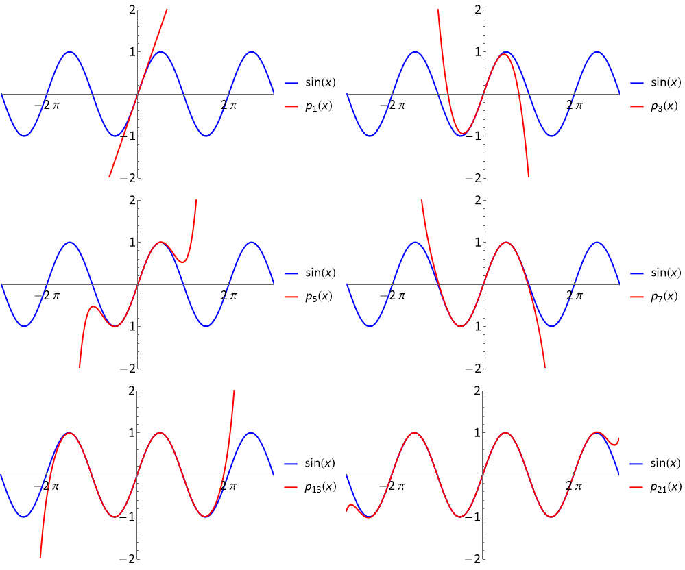
Fig. 5.1 A plot of the curve \(\sin(x)\) together with Maclaurin series expansion retaining successively greater numbers of terms, \(p_1,p_3,p_5,p_7,p_{13},p_{21}\).
As we can see. the degree 21 Maclaurin expansion represents \(\sin(x)\) rather faithfully in the range \([-2\pi,2\pi]\), but it is less accurate further away from the expansion point.
Worked example
Lets find the Taylor expansion of \(f(x)=e^x\) about \(x=0\) i.e. the Maclaurin series. We first need to find the derivatives, which here is easy:
Therefore the series looks like:
Notice that this series satisfies \(\displaystyle \frac{\mathrm{d}p}{\mathrm{d}x}=p\), which we would expect for \(p = e^x\).
An alternative derivation
A different way to derive the Taylor series of a function can be found by thinking about integration, if we apply the fundamental theorem of calculus:
Integrating by parts, we find:
We can then apply integration by parts repeatedly we find an infinite series for \(f(x)\) around \(x = 0\):
If we want to generalise this to any point \(x=a\), then we start with \(\displaystyle \int_0^{x-a} f'(x-t)\,\text{d}t\) :
The Maclaurin expansions of \(\sin\), \(\cos\), \(e^x\), and \(\ln(1+x)\) are particularly important:
You should also be able to calculate the first few terms in the expansion of an arbitrary function \(f(x)\).
Pratice questions
1. By regrouping the terms in the Maclaurin series for \(e^{i\theta}\), derive Euler’s formula.
2. Find the Maclaurin series for \(\cosh(x)\), giving your answer in the form of an infinite series.
3. Find the first two non-zero terms in the Maclaurin series for \(\textrm{arsinh}(x)\).
4.
a. Find the coefficient of \(x^n\) in the Maclaurin series expansion for \((x + 1)^{1/k},\,k,\, n \in \mathbb{N}, \,n > 2\).
b. Write the coefficient of \(x^6\) in the Maclaurin series of \((x+1)^{1/7}\) as an exact, proper fraction.
Solutions
1.
We can write this out rigorously as follows:
2. Let \(f(x) = \cosh(x)\), then:
Thus we find that for \(f^(n)\):
Hence the Taylor series is found from:
3. Let \(f(x) = \textrm{arsinh}(x)\)
Hence the Taylor series is given by:
4.
a. For \(f(x) = (x + 1)^{1/k}\), then we find:
Hence the \(n^{th}\) term will be found from:
b. We need to find \(c_{(7,\,6)}\):
A disclaimer!
Not all functions are faithfully represented by their Taylor Series. We have only guaranteed that the polynomial has the “correct” behaviour in the immediate vicinity of the point \(x=a\). Two things should be checked:
1. Does the series converge to a finite value for all \(x\)? - If not then it is important to find the radius of convergence. This can be achieved by using the ratio test
2. Does it converge to \(f(x)\)? - Even if the series converges, there is no guarantee that it converges to \(f(x)\). We would need to show that \(\displaystyle \lim_{k\rightarrow \infty}|f(x)-p_k(x;a)|=0\), which may only be true for some values of \(x\). (This can be done by making use of the Lagrange remainder theorem.)
Functions which converge to their Taylor series for a range of values are called analytic, and functions which converge to their Taylor series everywhere are called entire. The Taylor series for functions like sine, cosine exponential are entire, but the Maclaurin series for \(\ln(1+x)\) is analytic for \(|x|<1\).
The Taylor series nearly always contains an infinite number of terms. To be of practical use in applications, we typically need to “truncate” the expansion, meaning that we retain only the terms up to a specified \(n^{\text{th}}\) power of \(x\).
Example: The two-term expansion
Let us examine what happens if we retain just the first two terms in the Taylor series:
This defines a straight line - \(y = f'(a)x + (f(a) - af'(a))\). Since the line passes through the point \((a, \,f(a))\) it touches the curve f(x) at the point \(x = a\). The line has slope \(f^{\prime}(a)\), which is the gradient of the curve at \(x = a\), therefore, the two-term Taylor series is just the tangent to the curve at \(x = a\). The tangent is the best possible approximation that we can obtain for the curve near the point \(x = a\) using only two terms.
As well as considering the validity of the infinite series, it is important to be able to determine how many terms in the series are needed for practical use. If the series converges very slowly, then it may not be much good!
5.6.1. Composite function expansion
Let \(P(x)\), \(Q(x)\), be two power series that converge to \(f(x)\) and \(g(x)\) respectively
Then:
\(aP(x) + bQ(x)\) converges to \(af(x)+ bg(x)\)
\( P(x)Q(x)\) converges to \(f(x)g(x)\)
\( P(Q(x))\) converges to \(f(g(x))\)
It means that we can construct the Taylor series for a composite function by using known results for elementary functions (although we need to take care to check the region of validity)