.md .pdf

repository open issue

Contents

10. Integration

10.1. Introducing Integration

10.1.1. The “anti-derivative”

Consider the function \(\cos(x)\). We know that this function can be obtained by differentiating \(\sin(x)\). Therefore, we could think of \(\sin(x)\) as the “anti-derivative” of \(\cos(x)\). After differentiating \(\sin(x)\), the “anti-derivative” takes us back to where we started.

Well… nearly. We could also obtain \(\cos(x)\) by differentiating \(\sin(x)+2\), so we cannot say that \(\sin(x)\) is the unique anti-derivative of \(f(x)\).

In general, for a given function \(f(x)\),

if \(\frac{\mathrm{d}F}{\mathrm{d}x} = f(x)\), then \(F(x)+c\) is an antiderivative of \(x\),

where \(c\) is an arbitrary constant.

Being able to “spot” anti-derivatives is a tremendously useful (and often under-utilised) trick.

Practice questions

Note: these are not “integration questions”, you only need to use your knowledge of differentiation, and the concept of the anti-derivative, as described above.

1. \(\sec^2(x)\)

2. \(x^3\)

3. \(\sin(3x)\)

4. \(e^{a x}\)

5. \(x \sqrt{x^2-1}\)

6. \(\frac{x}{x^2+1}\)

7. \(\displaystyle \frac{\sin(x)}{\cos(x)}\)

8. \(\cosh(x)\sinh^2(x)\)

Solutions

1. We should recognise that \(\sec^2(x)\) is obtained by differentiating \(\tan(x)\) and so the anti-derivative is \(F(x)=\tan(x)+c\).

2. If we differentiate \(x^4\) we obtain \(4x^3\) which is nearly what we want, but not quite. Trying \(\displaystyle \frac{\mathrm{d}}{\mathrm{d}x} \left(\frac{1}{4} x^4\right)\) instead gets the result \(x^3\) and so the anti-derivative of \(x^3\) is \(\displaystyle \frac{1}{4} x^4+c\).

3. By the chain rule, \(\frac{\mathrm{d}}{\mathrm{d}x} \cos(3x)=-3\sin(3x)\), and so the anti-derivative is \(\displaystyle -\frac{1}{3}\cos(3x)+c\).

4. Since \(\displaystyle \frac{\mathrm{d}}{\mathrm{d}x}e^{a x}=a e^{a x}\) and so the anti-derivative is \(\displaystyle \frac{1}{a} e^{a x}+c\).

5. Now we rely on our expertise with the chain rule.

The chain rule tells us that \(f(g(x))^{\prime}=g^{\prime}(x)f^{\prime}(g)\) and so the anti-derivative of \(g^{\prime}(x)f^{\prime}(g)\) is \(f(g(x))+c\). In particular, if we differentiate \(g^{3/2}\) where \(g=x^2-1\), we obtain \((2 x) \frac{3}{2} g^{1/2}\) and so the anti-derivative of \(x g^{1/2}\) is

\[\frac{1}{3} g^{3/2}+c =\frac{1}{3} (x^2-1)^{3/2}+c\]

CHECK YOUR ANSWER: you need to be awesome at differentiation to be good at integration!

6. By the same rationale as question 5, we try \(\displaystyle \frac{\mathrm{d}}{\mathrm{d}x} \ln(x^2+1)=\frac{2x}{x^2+1}\) and so the anti-derivative is \(\displaystyle \frac{1}{2} \ln(x^2+1)+c\).

7. The anti-derivative is \(\displaystyle -\ln(\cos(x))+c\). In general, the anti-derivative of an expression of the form \(\displaystyle \frac{f^{\prime}(x)}{f(x)}\) is \(\ln(f(x))+c\).

8. The anti-derivative is \(\displaystyle \frac{1}{3} \sinh^3(x)+c\).

10.1.2. Area under the curve

Definition

Fig. 10.1 shows how the area under a curve \(f(x)\) between \(x=a,b\) may be estimated by drawing rectangles of equal width \(\Delta x\). Formally, we may write that:

(10.1)\[\textrm{Area} = \sum_{j=0}^{n-1}f(x_n)\Delta x \textrm{, where }x_0=a, x_n=b, \Delta x = \frac{b-a}{n}\]

The expression simply states that we add up the rectangles with width \(\Delta x\) and height \(f(x_n)\). As \(\Delta x\rightarrow 0\) the area approximation becomes more accurate.

We call:

\[\lim_{\Delta x \rightarrow 0}\sum_{j=0}^{n-1}f(x_j)\Delta x\]

the integral of \(f\) with respect to \(x\) and we denote it by:

(10.2)\[ \displaystyle \int_a^b f(x)\mathrm{d}x\]

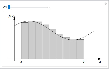
Fig. 10.1 Rectangles drawn under the curve \(f(x)\) can be used to approximate the area. The thinner the rectangles, the better the approximation. Integration is the equivalent to this approach as the width of the rectangles, \(\Delta x \rightarrow 0\).

It can be proved that integration and anti-differentiation are essentially the same thing. This result is known as the Fundamental Theorem of Calculus. In fact, the theorem comes in two parts. The first part, given in the box below, allows the definite integral to be determined by evaluating an anti-derivative at integration limits. The second part (not given here) essentially proves that every continuous function has an anti-derivative, which can be found by integration. For some functions, such as \(e^{-x^2}\), we might not be able to express the integral in terms of elementary functions, but we know it exists (and we can use successive approximation techniques either analytically or numerically to estimate them).

Definition

The First Fundamental Theorem of Calculus (FTC1)

If \(F\) is an anti-derivative of \(f\), then \(\displaystyle \int_a^b f(x) \textrm{d}x = F(b) - F(a)\) gives the area between the curve \(f(x)\) and the x-axis between \(x=a\) and \(x=b\).

Symbol	Meaning	Notes
\(\textrm{d}x\)	“with respect to x” The integration is along the x-axis. We say that x is the “integration variable”	Do not forget to write this, or the integral has no meaning.
\(\displaystyle \int\)	Integration operator	An operator acs on a function in some way. For example, \(\frac{\textrm{d}}{\textrm{d}x}\) is also an operator.
\(f(x)\)	Integrand	The function to be integrated.
\(a, b\)	The limits of integration.	If the integral has limits then it is called a definite integral and has a single value for the solution. If the integration does not have limits then it is called an indefinite integral, and you can only compute the result to within an arbitrary constant.

10.1.3. Signed and unsigned areas

Note that the heights of the rectangles in Fig. 10.1 are given by \(f(x)\), and so if \(f(x)<0\) then the result will be negative. In many examples, positive and negative areas cancel. For instance,

(10.3)\[\displaystyle \int_0^{2\pi}\sin(x)\mathrm{d}x = 0 \textrm{, since } \displaystyle \int_0^{\pi}\sin(x)\mathrm{d}x = 2 \textrm{ and } \displaystyle \int_{\pi}^{2\pi}\sin(x)\mathrm{d}x = -2\]

If you want the total (unsigned) area between the curve and the axis, then you can work with the modulus of the function,

(10.4)\[\displaystyle \int_a^b |f(x)|\mathrm{d}x\]

The easiest way to do this is to split up the region of integration into areas where \(f(x)>0\) and areas where \(f(x)<0\). For example,

(10.5)\[\displaystyle \int_0^{2\pi}|\sin(x)|\mathrm{d}x = \displaystyle \int_0^{\pi}\sin(x)\mathrm{d}x+ \displaystyle \int_{\pi}^{2\pi}-\sin(x)\mathrm{d}x = 2+2 =4\]

The results are illustrated in Fig. 10.2:

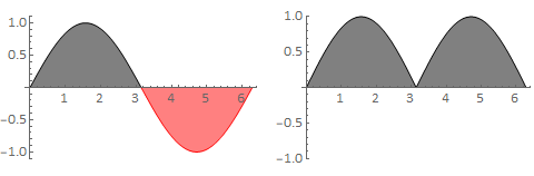
Fig. 10.2 The plot on the left shows \(\sin(x)\) for \(x\in[0,2\pi]\). The black and red signed areas (2,-2) cancel when the integral is performed. The plot on the right shows \(|\sin(x)|\) for \(x\in[0,2\pi]\). The black signed are both positive and so the integral is 2+2=4.

Similarly, if we perform the integration along the x-axis in the negative direction, then the quantities \(\Delta x\) are negative, and so we end up with a negative signed area when \(f(x) > 0\).

FTC1 also confirms that \(\displaystyle \int_b^a f(x) \textrm{d}x = -\displaystyle \int_a^b f(x) \textrm{d}x\).

10.1.4. Area between two curves

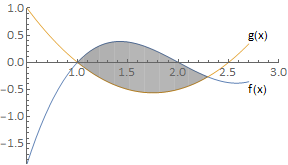
Fig. 10.3 Where \(f(x) >= g(x)\) the integral \(\displaystyle \int (f(x)-g(x)) \textrm{d}x\) gives the area between the two curves.

Practice questions

1. a. Find the tangent to the curve \(y=25-x^2\) at the point where \(x=2\).

b. Calculate the value of \(x\) where the tangent meets the x-axis.

c. Find the area of the region bounded by the tangent, the curve and the x-axis.

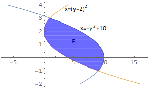
2. Calculate the area of the region bounded by the curves \(x = -y^2 + 10\) and \(x = (y-2)^2\).

Solutions

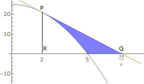
The tangent is \(y=29-4x\), which intersect that x-axis at \(x=29/4\) see diagram Q2:

The required area is given by PQR:

\[\int_2^5(25-x^2)\mathrm{d}x = \frac{1}{2}\left(\frac{21}{4}21 - \left[25x-\frac{x^3}{3}\right]_2^5\right) = \frac{153}{8}\]

The curves intersect at (1,3) and (9,-1) and it is easier to calculate the enclosed area by integrating parallel to the y-axis.

\[R = \int_{y=1}^3\left[(10-y^2)-(y-2)^2\right]\mathrm{d}y = \int_1^3(-2y^2+4y+6)\mathrm{d}y =\frac{64}{3}\]

10.2. Integration by substitution

Definition

For an indefinite integral:

\[\int f(x) \textrm{d}x = \int f(x) \frac{\mathrm{d}x}{\mathrm{d}u}\mathrm{d}u+c\]

For a definite integral:

\[\int_a^b f\mathrm{d}x= \int_{u(a)}^{u(b)}f\frac{\mathrm{d}x}{\mathrm{d}u}\mathrm{d}u\]

Don’t forget to change the limits for definite integration!

These results can be proved using the chain rule and fundamental theorem of calculus.

The idea of using a substitution is that we convert a difficult integral w.r.t \(x\) to an easier one w.r.t \(u\).

Note that \(\displaystyle f \frac{\mathrm{d}x}{\mathrm{d}u}=f\biggr/\frac{\mathrm{d}u}{\mathrm{d}x}\) and so the substitution \(u\) can be chosen to eliminate a factor from \(f\).

Worked example

To calculate \( \displaystyle \int x\sqrt{x^2-1}\mathrm{d}x\) we can try the substitution \(u=x^2-1\). This substitution will eliminate the factor \(x\) and will simplify the expression \(\sqrt{x^2-1}\). We find that:

\(\displaystyle \frac{\mathrm{d}u}{\mathrm{d}x}=2x\) and so \(\displaystyle \frac{\mathrm{d}x}{\mathrm{d}u}=\frac{1}{2x}\), hence:

\[\int x\sqrt{x^2-1}\mathrm{d}x=\displaystyle \int\frac{1}{2}u^{1/2}\mathrm{d}u=\frac{1}{3}u^{3/2}+c=\frac{1}{3}(x^2-1)^{3/2}+c\]

This is the same result we can find by inspection.

Practice questions

1. Find \( I= \displaystyle\int_1^3\frac{1}{2x+1}\mathrm{d}x\).

2. Find \( I= \displaystyle\int (ax+b)(cx+d)^n\mathrm{d}x\) using the substitution \(u=cx+d\),/

Solutions

1. To calculate the definite integral \( I=\displaystyle \int_1^3\frac{1}{2x+1}\mathrm{d}x\), we will use the substitution \(u=2x+1\). (This problem could also be solved by inspection).

When \(x=1\), \(u=3\) and when \(x=3\), \(u=7\), hence, the result is

\[\begin{split}I&=\int_{u=3}^{u=7}\frac{1}{u}\biggr/\frac{\mathrm{d}u}{\mathrm{d}x}\mathrm{d}u \\ &=\frac{1}{2} \int_3^7\frac{1}{u}\mathrm{d}u=\frac{1}{2}\biggr[\ln(u)\biggr]_3^7=\frac{1}{2}\ln\biggr(\frac{7}{3}\biggr)\end{split}\]

2. To calculate an expression of the form \( I=\displaystyle \int (ax+b)(cx+d)^n\mathrm{d}x\) we can make the substitution \(u=cx+d\), which gives:

\[I=\int\left(a\frac{u-d}{c}+b\right)u^n\frac{1}{c}\mathrm{d}u=\frac{1}{c^2}e \int(au+bc-ad)u^n\mathrm{d}u\]

By polynomial expansion:

\[I=\frac{1}{c^2}\int(a u^{n+1}+(bc-ad)u^n)\mathrm{d}u=\frac{1}{c^2}\left[\frac{a u^{n+2}}{n+2}+\frac{bc-ad}{n+1}u^{n+1}\right]\]

Rewriting in terms of \(x\) finally gives:

\[I = \frac{(cx+d)^{n+1}}{c^2}\left[\frac{a(cx+d)}{n+2}+\frac{bc-ad}{n+1}\right]\]

10.3. Integral of \(\displaystyle \frac{1}{x}\)

The function \(\displaystyle \frac{1}{x}\) falls into a special category, because it cannot be solved using the polynomial antiderivative \(\displaystyle \int x^n = \frac{x^{n+1}}{n+1}\) as \(n=-1\) here.

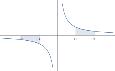
Fig. 10.4 The plot of \(\displaystyle y=\frac{1}{x}\), showing limits of integration \(\pm a\) and \(\pm b\).

However we can think about the fact that \(\displaystyle \frac{\mathrm{d}}{\mathrm{d}x}\Big(\ln(x)\Big) = \frac{1}{x}\) and therefore use this as an antiderivative. From Fig. 10.4, we see that:

\[\int_{-b}^{-a}\frac{1}{x}\mathrm{d}x = -\int_a^b\frac{1}{x}\mathrm{d}x = \int_b^a\frac{1}{x}\mathrm{d}x = \int_{-b}^{-a}\frac{1}{|x|\mathrm{d}x}\]

So, \(\displaystyle \int\frac{1}{x}=\ln(|x|)+\mathrm{const},\, \forall x\), provided that the range of integration does not cross the vertical axis.

This is because formally \(\displaystyle \int_{-a}^a\frac{1}{x}\mathrm{d}x\) is undefined, although we can define what is called the Cauchy principal value of this integral as:

\[\lim_{\epsilon\rightarrow 0^{+}}\left( \int_{-a}^{-\epsilon}\frac{1}{x}\mathrm{d}x+ \int_{\epsilon}^a\frac{1}{x}\mathrm{d}x\right)=0\]

10.4. Integration by parts

Definition

For an indefinite integral:

\[\int u\,\frac{\mathrm{d}v}{\mathrm{d}x}\,\mathrm{d}x = u\,v- \int v\,\frac{\mathrm{d}u}{\mathrm{d}x}\,\mathrm{d}x+c\]

For a definite integral:

\[\int_a^b u\,\frac{\mathrm{d}v}{\mathrm{d}x}\,\mathrm{d}x=\biggr[u\,v\biggr]_a^b- \int_a^b v\frac{\mathrm{d}u}{\mathrm{d}x}\,\mathrm{d}x\]

This result can be proved using the product rule and the fundamental theorem of calculus.

\[\begin{split}\mathrm{d}(u\,v) &= u\,\mathrm{d}\,v + v\,\mathrm{d}u \\ u\,\mathrm{d}\,v &= \mathrm{d}(u\,v) - v\,\mathrm{d}u \\ \int u\,\mathrm{d}\,v &= \int \mathrm{d}(u\,v) - \int v\,\mathrm{d}u \\ \Rightarrow \int u\,\mathrm{d}\,v &= u\,v - \int v\,\mathrm{d}u\end{split}\]

For a handy rule of thumb for choosing which term to differentiate when applying this method, we can use LIATE method:

• Logarithmic Term

• Inverse Term

• Algebraic Term

• Trignometric Term

• Exponential Term

This list tells the order of preference for the term to be differentiated \(u(x) \rightarrow u'(x)\). The exponential function is at the bottom of the sit because it is usually the easiest to integrate, the logarithmic is usually the hardest, hence it sits at the top.

Worked Examples

1.

\[I_a = \int x \ln(x)\,\mathrm{d}x \]

Since L falls before A in LIATE, we pick:

\[\begin{split}u = \ln(x),\quad & v' = x\\ u' = \frac{1}{x}, \quad & v = \frac{1}{2}x^2\end{split}\]

and so integrating by parts we find:

\[I_a = \frac{1}{2} \,x^2 \,\ln(x) - \int \frac{1}{2} \,x \,\mathrm{d}x = \frac{1}{2} \, x^2 \left(\ln(x) - \frac{1}{2} \right) + C\]

2. Sometimes it is not always obvious that there are two functions in the integration expression, however this can be remedied using a simple trick:

\[I_b = \int \ln(x)\,\mathrm{d}x \]

This should be seen as:

\[I_b = \int x^0\,\ln(x)\,\mathrm{d}x \]

Since L falls before A in LIATE, we pick:

\[\begin{split}u = \ln(x),\quad & v' = x^0 \\ u' = \frac{1}{x},\quad &v = x^1\end{split}\]

and so integrating by parts we find:

\[I_b = x \ln(x) - \int \frac{x}{x}\,\mathrm{d}x = x\ln(x) - \int x^0\,\mathrm{d}x = x\ln(x) - x + C \]

Practice Problems

Integrate the following problems by parts:

1.

\[\int x e^{-x}\mathrm{d}x\]

2.

\[\int x^2 e^{-x}\mathrm{d}x\]

3.

\[I= \int \arcsin(x)\mathrm{d}x\]

Solutions

1. To calculate \(\displaystyle \int x e^{-x}\mathrm{d}x\),

Let \(u=x,\ v'=e^{-x}\) then:

\(u'=1\), which is simpler and \(v=-e^{-x}\) which is no more complicated, so:

\[\int x e^{-x}\mathrm{d}x = -x e^{-x}+ \int e^{-x}\mathrm{d}x = -e^{-x}(x+1)+C\]

2. To calculate \(\displaystyle \int x^2 e^{-x}\mathrm{d}x\),

Let \(u=x^2,\, v'=e^{-x}\), then:

\(u'=2x\), which is simpler and \(v=-e^{-x}\), which is no more complicated, so:

\[\int x^2 e^{-x}\mathrm{d}x=-x^2 e^{-x}+2\int x e^{-x}\mathrm{d}x\]

From the previous example, we know the result of this integrand is:

\[\int x e^{-x}\mathrm{d}x = -e^{-x}(x+1)+C\]

and therefore we find:

\[ \int x^2 e^{-x}\mathrm{d}x=-e^{-x}(x^2+2x+2)\]

3. To calculate \( I =\displaystyle \int \arcsin(x)\mathrm{d}x\) we play a trick:

Let \(u=\arcsin(x)\), \(v'=1\), then:

\(x=\sin(u)\), so \(\displaystyle \frac{\mathrm{d}x}{\mathrm{d}u}=\cos(u)=\pm\sqrt{1-x^2}\)

We should be cautious here because of the \(\pm\) - the positive square root is chosen because \(\sin(x)\) is increasing throughout its domain.

Also we have \(v=x\), so this gives

\[I=x\arcsin(x)- \int\frac{x}{\sqrt{1-x^2}}\mathrm{d}x\]

The remaining integral can be calculated by inspection, or with the substitution \(g=1-x^2\):

\[I=x \arcsin(x)+\sqrt{1-x^2}+C\]

10.5. Integration by partial fractions

Composing fractions means putting everything together, such as:

\[\frac{A}{x+a} + \frac{B}{x+b} = \frac{(A+B)x + (Ab+Ba)}{(x+a)(x+b)}\]

Decomposition is the reverse process, i.e. taking the fraction apart. This very useful for integration, since the resulting partial fractions are much easier to integrate to logarithmic type terms.

We can combine together our facts about partial fractions into:

Factor in denominator	Term in partial fraction decomposition
\(ax+b\)	\(\displaystyle \frac{A}{ax+b}\)
\((ax+b)^n\)	\(\displaystyle \frac{A_1}{ax+b} + \frac{A_2}{(ax+b)2} + \dots \frac{A_n}{(ax+b)^n}, \quad n \in \mathbb{N}\)
\(ax^2+bx+c\)	\(\displaystyle \frac{Ax+B}{ax^2+bx+c}\)
\((ax^2+bx+c)^n\)	\(\displaystyle \frac{A_1}{ax^2+bx+c} + \frac{A_2}{(ax^2+bx+c)^2} + \dots \frac{A_n}{(ax^2+bx+c)^n}, \quad n \in \mathbb{N}\)

Worked example

Find the value of the integral

\[\int \frac{5x+7}{x^2+3x+2}\,\mathrm{d}x\]

Since this is an algebraic fraction we can try to express as partial fractions:

\[\begin{split}\frac{5x+7}{x^2+3x+2} &= \frac{5x+7}{(x+1)(x+2)}\\ &= \frac{A}{x+1}+\frac{B}{x+2} = \frac{A(x+2) + B(x+1)}{(x+1)(x+2)}\\ &= \frac{(A+B)x + 2A+B}{(x+1)(x+2)} \\ \Rightarrow 5x + 7 &= (A+B)x + 2A+B\end{split}\]

Which leads to simultaneous equations:

\[\begin{split}A + B &=5 \\ 2A + B &= 7\end{split}\]

and is solved by \(A = 2,\, B = 3\), therefore:

\[\begin{split}\frac{5x+7}{x^2+3x+2} &= \frac{2}{x+1}+\frac{3}{x+2} \\ \, \\ \int \frac{5x+7}{x^2+3x+2}\,\mathrm{d}x &= 2\ln|x+1| + 3\ln|x+2| + C\end{split}\]

Practice questions

Evaluate the following integrals:

1.

\[\int\frac{3x+11}{x^2-x-6}\,\mathrm{d}x\]

2.

\[\int\frac{x^2+4}{3x^3+4x^2-4x}\,\mathrm{d}x\]

3.

\[\int\frac{x^2-29x+5}{(x-4)^2(x^2+3)}\,\mathrm{d}x\]

4.

\[\int\frac{x^3+10x^2+3x+36}{(x-1)(x^2+4)^2}\,\mathrm{d}x\]

5.

\[\int\frac{x^4-5x^3+6x^2-18}{x^3-3x^2}\,\mathrm{d}x\]

6.

\[\int\frac{x^3}{x^2-1}\,\mathrm{d}x\]

Solutions

1.

\[\begin{split}\frac{3x+11}{x^2-x-6} &= \frac{A}{x-3} + \frac{B}{x+2} = \frac{A(x+2)+B(x-3)}{x^2-x-6} \\ \Longrightarrow &A(x+2)+B(x-3) = 3x+11 \\ x=-2: &\qquad A(0) + B(-5) = 5 \Rightarrow B = -1 \\ x=3: &\qquad A(5) + B(0) = 20 \Rightarrow A = 4 \\ \int\frac{3x+11}{x^2-x-6}\,\mathrm{d}x &=\int\left(\frac{4}{x-3} - \frac{1}{x+2}\right)\,\mathrm{d}x\\ &= 4\ln|x-3| - \ln|x+2| + K\end{split}\]

2.

\[\begin{split}\frac{x^2+4}{3x^3+4x^2-4x} &= \frac{x^2+4}{x(x+2)(3x-2)}= \frac{A}{x} + \frac{B}{x+2} + \frac{C}{3x-2} \\ &= \frac{A(x+2)(3x-2) + Bx(3x-2) + Cx(x+2)}{x(x+2)(3x-2)} \\ \Longrightarrow & A(x+2)(3x-2) + Bx(3x-2) + Cx(x+2) = x^2+4 \\ x=0: &\qquad A(2)(-2) + B(0) + C(0) = 4 \Rightarrow A = -1 \\ x=-2: &\qquad A(0) + B(-2)(-8) + C(0) = 8 \Rightarrow B = \frac{1}{2} \\ x=\frac{2}{3}: &\qquad A(0) + B(0) + C\left(\frac{2}{3}\right)\left(\frac{8}{3}\right) = \frac{40}{9} \Rightarrow C = \frac{5}{2} \\ \int\frac{x^2+4}{3x^3+4x^2-4x}\,\mathrm{d}x &=\int\left(-\frac{1}{x} + \frac{1}{2}\frac{1}{x+2} + \frac{5}{2}\frac{1}{3x-2}\right)\,\mathrm{d}x\\ &= -\ln|x| +\frac{1}{2} \ln|x+2| + \frac{5}{6}\ln|3x-2|+ K\end{split}\]

3.

\[\begin{split}\frac{x^2-29x+5}{(x-4)^2(x^2+3)} &= \frac{A}{x-4} + \frac{B}{(x-4)^2} + \frac{Cx+D}{x^2+3} \\ &= \frac{A(x-4)(x^2+3) + B(x^2+3) + (Cx+D)(x-4)^2}{(x-4)^2(x^2+3)} \\ \Longrightarrow & A(x-4)(x^2+3) + B(x^2+3) + (Cx+D)(x-4)^2 = x^2-29x+5 \end{split}\]

Comparing coefficients at reach order in \(x\):

\[\begin{split}x^3: &\qquad A+C = 0 \\ x^2: &\qquad -4A + B - 8C + D = 1 \\ x^1: &\qquad 3A + 16C- 8D = -29 \\ x^0: &\qquad -12A + 3B + 16D = 5 \\ &\Longrightarrow A = 1,\quad B = -5, \quad C = -1, \quad D = 2\\ \int\frac{x^2-29x+5}{(x-4)^2(x^2+3)}\,\mathrm{d}x &=\int\left(\frac{1}{x-4} - \frac{5}{(x-4)^2} + \frac{2-x}{x^2+3}\right)\,\mathrm{d}x\\ &= \int\left(\frac{1}{x-4} - \frac{5}{(x-4)^2} + \frac{2}{x^2+3} - \frac{x}{x^2+3}\right)\,\mathrm{d}x\\ &= \ln|x-4| + \frac{5}{x-4} + \frac{2}{\sqrt{3}}\arctan\left(\frac{x}{\sqrt{3}}\right)- \frac{1}{2}\ln|x^2+3|+ K\end{split}\]

4.

\[\begin{split}\frac{x^3+10x^2+3x+36}{(x-1)(x^2+4)^2} &= \frac{A}{x-1} + \frac{Bx+C}{(x^2+4)} + \frac{Dx+E}{(x^2+4)^2} \\ &= \frac{A(x^2+4)^2 + (Bx+C)(x-1)(x^2+4) + (Dx+E)(x-1)}{(x-1)(x^2+4)^2} \\ \Longrightarrow A(x^2+4)^2 &+ (Bx+C)(x-1)(x^2+4) + (Dx+E)(x-1) = x^3+10x^2+3x+36\end{split}\]

Comparing coefficients at reach order in \(x\):

\[\begin{split}x^4: &\qquad A + B = 0 \\ x^3: &\qquad C - B = 1 \\ x^2: &\qquad 8A + 8B - C + D = 10 \\ x^1: &\qquad -4B + 4C - D + E = 3 \\ x^0: &\qquad 16A - 4C -E = 36 \\ &\Longrightarrow A = 2,\quad B = -2, \quad C = -1, \quad D = 1, \quad E = 0\\ \int\frac{x^3+10x^2+3x+36}{(x-1)(x^2+4)^2}\,\mathrm{d}x &=\int\left(\frac{2}{x-1} - \frac{2x+1}{(x^2+4)} + \frac{x}{(x^2+4)^2} \right)\,\mathrm{d}x\\ &= \int\left(\frac{2}{x-1} - \frac{2x}{(x^2+4)} + \frac{1}{(x^2+4)} + \frac{x}{(x^2+4)^2} \right)\,\mathrm{d}x\\ &= 2\ln|x-1| - \ln|x^2 + 4| + \frac{1}{2}\arctan\left(\frac{x}{2}\right)- \frac{1}{2}\frac{1}{x^2+4}+ K\end{split}\]

5. Since this is a top heavy fraction, we should try to cancel this down first:

\[\begin{split}\frac{x^4-5x^3+6x^2-18}{x^3-3x^2} &= \frac{x^4 - 3x^3 + 3x^3 - 5x^3 + 6x^2 - 18}{x^3-3x^2} \\ &= x + \frac{-2x^3 + 6x^2 - 18}{x^3-3x^2} = x + \frac{-2x^3 + 6x^2} - \frac{18}{x^3-3x^2}\\ &= x - 2 - \frac{18}{x^3-3x^2} = x - 2 - \frac{18}{x^2(x-3)}\\ \frac{18}{x^2(x-3)} &= \frac{A}{x} + \frac{B}{x^2} + \frac{C}{x-3} = \frac{Ax(x-3) + B(x-3) + Cx^2}{x^2(x-3)}\\ x=0: &\qquad A(0) + B(-3) + C(0)= 18 \Rightarrow B = -6 \\ x=3: &\qquad A(0) + B(0) + C(9) = 18 \Rightarrow C = 2 \\ x=1: &\qquad A(-2) + B(-2) + C(1) = 18 \Rightarrow A = -2 \\ \int\frac{x^4-5x^3+6x^2-18}{x^3-3x^2}\,\mathrm{d}x &= \int\left(-\frac{2}{x} - \frac{6}{x^2} + \frac{2}{x-3}\right)\,\mathrm{d}x\\ &= \frac{1}{2}x^2 - 2x + 2\ln|x| - \frac{6}{x} - 2\ln|x-3| + K\end{split}\]

6.

\[\begin{split}\frac{x^3}{x^2-1} &= \frac{x^3-x^2 + x^2 - 1 + 1}{x^2-1} = x + 1 + \frac{1}{x^2-1} = x + 1 + \frac{1}{(x-1)(x+1)}\\ &= x + 1 + \frac{1}{2}\left(\frac{1}{x-1} - \frac{1}{x+1}\right)\\ \int\frac{x^3}{x^2-1}\,\mathrm{d}x &= \int\left[x + 1 + \frac{1}{2}\left(\frac{1}{x-1} - \frac{1}{x+1}\right)\right]\,\mathrm{d}x\\ &= \frac{1}{2}x^2 + x + \frac{1}{2}\ln|x-1| - \frac{1}{2}\ln|x+1| + K\end{split}\]

10.6. Reduction formula

Reduction formulae set up a recurrence relation between different integrands:

\[I_{n} = f(n,x) + I_{n-a} \]

where \(a,\,n\) are integers typically and \(a < n\). Usually we solve these problems by integration by parts, which by spotting the required pattern, makes finding the solution more straightforward.

Worked example

Find and evaluate the reduction formula for:

\[I_n = \int_0^\infty x^n\,e^{-x}\,\mathrm{d} x\]

We can integrate by parts (using LIATE if necessary):

\[\begin{split}\begin{array}{lcl} u(x) = x^n && v'(x) = e^{-x} \\ u'(x) = nx^{n-1} && v(x) = -e^{-x} \end{array}\end{split}\]

Which means that we can write:

\[\begin{split}I_n &= \bigg[-x^n\,e^{-x}\bigg]_0^\infty + n\int_0^\infty x^{n-1}\, e^{-x}\,\mathrm{d} x \\ I_n &= 0 + n I_{n-1}\end{split}\]

If we were to repeat the integration by parts repeatedly we would find:

\[I_n = nI_{n-1} = n(n-1)\,I_{n-2} = \dots = n(n-1)(n-2)\dots (2)(1)\,I_0 = n!\, I_0\]

\(I_0\) is a good place to stop, since we can evaluate it:

\[I_0 = \int_0^\infty e^{-x}\,\mathrm{d} x = \bigg[-e^{-x}\bigg]_0^\infty = 0 - (-1) = 1\]

Hence \(I_n = n!\).

Practice Questions

1. Find a reccurence relation for the integral:

\[I_n = \int x^n e^x\mathrm{d}x\]

and find a value for \(I_4\).

2. Find a reccurence relation for the integral:

\[I_n = \int_0^{\pi/2}\cos^{n}(x)\mathrm{d}x \]

and find a value for \(I_{10}\).

3. Find the reduction formula for:

\[I_n = \int_0^1 (1 - x^3)^n\,\mathrm{d} x\]

and evaluate \(I_4\).

4. Find the reduction formula for:

\[I_n = \int_0^{\pi/2} \sin^n(x)\,\mathrm{d} x \]

and evaluate \(I_2, \, I_3\).

Solutions

1.

\[I_n = \int x^n e^x\mathrm{d}x \]

Integrating by parts:

\[\begin{split}\begin{array}{lcl} u(x) = x^n && v'(x) = e^x \\ u'(x) = nx^{n-1} && v(x) = e^x \end{array}\end{split}\]

and therefore:

\[I_n = \int x^n e^x\mathrm{d}x = x^n e^x - n \int x^{n-1}e^x\mathrm{d}x\]

Hence the reccurence relation is

\[I_n = x^n e^x - n I_{n-1}\]

Which means that:

\[I_0 = \displaystyle \int e^x\mathrm{d}x = e^x + C\]

and so \(I_4\) is given by:

\[\begin{split}I_4 &= e^x(x^4- 4x^3+4(3)x^2 - 4(3)(2)x +4(3)(2)(1))+C\\ &= e^x(x^4- 4x^3+12x^2 - 24x +24)+C\end{split}\]

2.

\[I_n = \int_0^{\pi/2}\cos^{n}(x)\mathrm{d}x = \int_0^{\pi/2}\cos(x)\cos^{n-1}(x)\mathrm{d}x\]

Integrating by parts:

\[\begin{split}\begin{array}{lcl} u(x)= \cos^{n-1}(x) && v'(x) = \cos(x) \\ u'(x) = -(n-1)\cos^{n-2}(x)\sin(x) && v(x) = \sin(x) \end{array}\end{split}\]

and therefore:

\[\begin{split}I_n &= \left[\sin(x)\cos^{n-1}(x)\right]_0^{\pi/2} + (n-1) \int_0^{\pi/2}\sin(x)\cos^{n-2}(x)\sin(x)\mathrm{d}x \\ &=(0-0)+(n-1)\displaystyle \int\sin^2\cos^{n-2}(x)\mathrm{d}x \\ &=(n-1)\displaystyle \int(1-\cos^2(x)\cos^{n-2}(x)\mathrm{d}x \\ &=(n-1)(I_{n-2}-I_n)\end{split}\]

Rearranging gives:

\[I_n = \frac{n-1}{n}I_{n-2}\]

and so for \(I_{10}\):

\[I_{10} = \frac{9}{10}I_8 = \frac{9}{10}\frac{7}{8}I_6 = \dots = \frac{9\times7\times5\times3\times1}{10\times8\times6\times4\times2}I_0\]

and finally:

\[I_0 = \int_0^{\pi/2}\mathrm{d}x = \frac{\pi}{2}\]

Thus:

\[I_{10} = \frac{63\pi}{256}\]

3. There may be a temptation to try to expand out the bracket or integrate by parts straight away, however the easier method is to break up the integrand into \((1-x^3)^{n-1}\,(1-x^3)\):

\[\begin{split}I &= \int_0^1 (1-x^3)^{n-1}\,\mathrm{d} x -\int_0^1 x^3\,(1-x^3)^{n-1}\,\mathrm{d} x \\ &= I_{n-1} - \int_0^1 x\,x^2\,(1-x^3)^{n-1}\,\mathrm{d} x \\ &= I_{n-1} - \int_0^1 x\,\left(-\frac{1}{3}\right)(-3x^2)\,(1-x^3)^{n-1}\,\mathrm{d} x \end{split}\]

and then integrate the second integrand by parts:

\[\begin{split}\begin{array}{lcl} u(x) = x && v'(x) = -\frac{1}{3} (-3x^2)(1-x^3)^{n-1}\\ u'(x) = 1 && v(x) = -\frac{1}{3n} (1-x^3)^{n} \end{array}\end{split}\]

where we integrated \(f'(x)\) using the reverse chain rule.

\[\begin{split}\Rightarrow I_n &= I_{n-1} - \bigg[ -\frac{x}{3n} (1-x^3)^{n}\bigg]_0^1 - \frac{1}{3n}\int_0^1 (1-x^3)^{n}\,\mathrm{d} x \\ I_n &= I_{n-1} + 0 - \frac{1}{3n}I_{n} \Longrightarrow I_n = \frac{3n}{3n+1}I_{n-1} \\ I_4 &= \bigg(\frac{12}{13}\bigg)I_3 = \bigg(\frac{12}{13}\bigg)\bigg(\frac{9}{10}\bigg)I_2 \\ &= \bigg(\frac{12}{13}\bigg)\bigg(\frac{9}{10}\bigg)\bigg(\frac{6}{7}\bigg)I_1 = \bigg(\frac{12}{13}\bigg)\bigg(\frac{9}{10}\bigg)\bigg(\frac{6}{7}\bigg)\bigg(\frac{3}{4}\bigg)I_0 \\ I_0 &= \int_0^1\mathrm{d} x = 1 \\ \Rightarrow I_4 &= \frac{243}{455} \end{split}\]

4. Firstly break up the integrand into \(\sin(x) \sin^{n-1}(x)\) and then integrate by parts:

\[\begin{split}\begin{array}{lcl} u(x) = \sin^{n-1}(x) && v'(x) = \sin(x) \\ u'(x) = (n-1)\cos(x)\sin^{n-2}(x) && v(x) = -\cos(x) \end{array}\end{split}\]

and therefore:

\[\begin{split}I_n &= \bigg[-\cos(x)\sin^{n-1}(x)\bigg]_0^{\pi/2} + (n-1)\int_0^{\pi/2} \cos^2(x) \sin^{n-2}(x)\,\mathrm{d} x \\ &= 0 + (n-1)\int_0^{\pi/2} (1 - \sin^2(x))\sin^{n-2}(x)\,\mathrm{d} x \\ &= (n-1)\int_0^{\pi/2} \bigg(\sin^{n-2}(x) - \sin^{n}(x)\bigg)\,\mathrm{d} x \\ I_n &= (n-1)I_{n-2} - (n-1)I_{n} \\ nI_n &= (n-1)I_{n-2} \\ \Rightarrow I_n &= \frac{n-1}{n}I_{n-2} \\ I_2 &= \frac{1}{2}I_0 = \frac{1}{2}\bigg[x\bigg]_0^{\pi/2} = \frac{\pi}{4}\\ I_3 &= \frac{2}{3}I_1 = \left(\frac{2}{3}\right)\bigg[-\cos(x)\bigg]_0^{\pi/2} = \frac{2}{3}\end{split}\]

notice we evaluate \(I_0\) and \(I_1\) depending on whether \(n\) is odd or even.

10.7. Mean value of a function

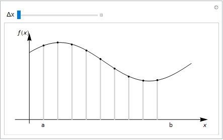
Fig. 10.5 The average of a discrete function is given by adding up the values and dividing by the number of points. We extend this concept to continuous functions in the limit as \(\Delta x\rightarrow 0\).

As shown in Fig. 10.5, for any function \(f(x)\) we can obtain the average output \(\bar{f(x)}\) by adding up a series of outputs and dividing by the number of datapoints used. In this case, the spacing between datapoints is \(\Delta x\).

\[\bar{f} = \frac{1}{n} \sum_{j=0}^{n-1}f(x_j) = \frac{\Delta x}{b-a}\sum_{j=0}^{n-1}f(x_j)\]

By taking the limit as \(\Delta x\rightarrow 0\), we can obtain an average of the function \(f(x)\) and we find that this result is equal to the limit defintion of the definite integral.

Definition

The mean value \(\bar{f}\) of the function \(f(x)\) on the domain \(x \in [a,\, b]\) is given by:

\[\bar{f} = \frac{1}{b-a} \int_a^b f(x)\mathrm{d}x\]

Worked example

Calculate the mean value of \(\cos ^3(\theta)\) on the interval \(\displaystyle \left[-\frac{\pi}{3}, \frac{\pi}{3}\right]\) by integration.

\[\begin{split}\frac{1}{\frac{\pi}{3} - \left(-\frac{\pi}{3}\right)} \int_{-\pi/3}^{\pi/3}\cos^{3}(\theta)\mathrm{d}\theta &= \frac{3}{2\pi}\displaystyle \int_{-\pi/3}^{\pi/3}\cos(\theta)(1-\sin^2(\theta))\mathrm{d}\theta\\ &=\frac{3}{2\pi}\left[\sin(\theta)-\frac{1}{3}\sin^3(\theta)\right]_{-\pi/3}^{\pi/3} = \frac{9\sqrt{3}}{8\pi}\end{split}\]

Practice questions

1. Find the average value of the function \(f(x) = x^3\) on the interval \(x \in [0,\, 1]\).

2. Find the mean value of the cosine function on the interval \(x \in \Big[0,\, \frac{\pi}{2}\Big]\).

Solutions

1.

\[\bar{f} = \frac{1}{1-0} \int_0^{1} x^3\,\mathrm{d}x = \int_0^{1} x^3\,\mathrm{d}x = \Big[ \frac{x^4}{4}\Big]_0^{1} = \frac{1}{4}\]

2.

\[\bar{f} = \frac{1}{\frac{\pi}{2}-0} \int_0^{\pi/2} \cos(x)\,\mathrm{d}x = \frac{2}{\pi} \int_0^{\pi/2} \cos(x)\,\mathrm{d}x = \frac{2}{\pi}\,\Big[ \sin(x)\Big]_0^{\pi/2} = \frac{2}{\pi}\]

10.8. Arc Length

Suppose that we have a function \(y = f(x)\), we know through integration that we can find the area under the curve:

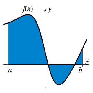
Fig. 10.6 The area (in blue) under a function \(f(x)\) over the interval \(x \in [a,\,b]\) given by the integral \(\displaystyle \int_a^bf(x)\,\mathrm(d)x\).

Another question that we could ask however is what is the length of the path traced out by the function \(f(x)\) over the range \([a,\,b]\):

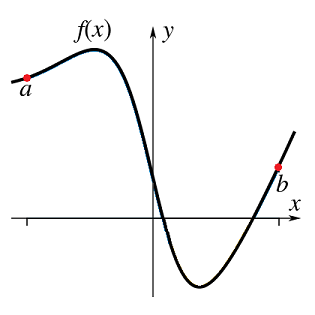
Fig. 10.7 The path traced out by the function \(f(x)\) over the interval \(x \in [a,\,b]\).

To find an expression for this length \(S\), we can break up the path into infinitesimal segments and then integrate these over the whole function. We can see this process breaking down the change in arc length \(\Delta s\) by Pythagoras graphically as:

\[(\Delta s)^2 = (\Delta x)^2 + (\Delta y)^2 \Rightarrow \Delta s = \sqrt{(\Delta x)^2 + (\Delta y)^2} = \Delta x\,\sqrt{1 + \left(\frac{\Delta y}{\Delta x}\right)^2}\]

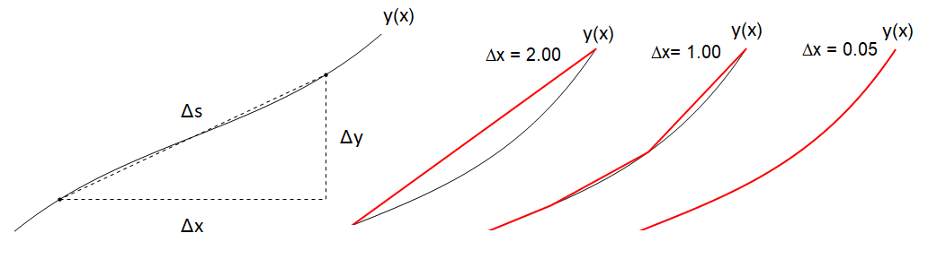
Fig. 10.8 Left Pane: Breaking down path legnth segment \(\Delta s\) into \(x,\, y\) components \(\Delta x,\, \Delta y\). The distance \(\Delta s\) moved along a curve, corresponding to small changes \(\Delta x \Delta y\) can be calculated by Pythagoras’ formula.

Right Pane: Effect of taking the limit of smaller \(\Delta x\) in finding the path length. By decreasing the difference \(\Delta x\) between the joined up points, we obtain a better approximation.

Taking the limit of \(\Delta x\rightarrow 0\) we find:

\[\mathrm{d}s = \mathrm{d}x\, \sqrt{1 + \left(\frac{\mathrm{d}y}{\mathrm{d}x}\right)^2}\]

and therefore to find the path length:

\[L = \int_{x=a}^{x=b} \mathrm{d}s = \int_a^b \sqrt{1 + \left(\frac{\mathrm{d}y}{\mathrm{d}x}\right)^2}\,\mathrm{d}x\]

We might also have a function which is parameterised \(y = y(t),\, x=x(t)\), it is also possible to find an expression for the path length for \(t \in [t_a,\, t_b]\), taking the limit of \(\Delta t \rightarrow 0\):

\[\begin{split}\Delta s &= \Delta t\,\sqrt{\left(\frac{\Delta x}{\Delta t}\right)^2 + \left(\frac{\Delta y}{\Delta t}\right)^2} \\ \Rightarrow \mathrm{d}s &= \mathrm{d}t\, \sqrt{\left(\frac{\mathrm{d}x}{\mathrm{d}t}\right)^2 + \left(\frac{\mathrm{d}y}{\mathrm{d}t}\right)^2}\\ L &= \int_{t_a}^{t_b} \sqrt{\left(\frac{\mathrm{d}x}{\mathrm{d}t}\right)^2 + \left(\frac{\mathrm{d}y}{\mathrm{d}t}\right)^2}\,\mathrm{d}t\end{split}\]

Worked examples

1. Looking at \(y = \cosh(x)\) over the range \(x \in [0,\,1]\), so we find \(\mathrm{d}y/\mathrm{d}x = \sinh(x)\), and therefore:

\[L = \int_0^1 \sqrt{1 + \sinh^2(x)}\,\mathrm{d}x = \int_0^1 \cosh(x)\,\mathrm{d}x = \Big[ \sinh(x) \Big]_0^1 = \sinh(1) \simeq 1.175\dots\]

2. Consider a circle, parameterised by \(x = R\cos(t),\, y = R\sin(t)\), over the range \(t \in [0,\, 2\pi)\), giving \(\mathrm{d}x/\mathrm{d}t = -R\sin(t),\, \mathrm{d}y/\mathrm{d}t = R\cos(t)\) and therefore:

\[L = \int_0^{2\pi} \sqrt{R^2\sin^2(t) + R^2\cos^2(t)}\,\mathrm{d}t = \int_0^{2\pi} R\,\mathrm{d}x = \Big[ Rt \Big]_0^{2\pi} = 2\pi\,R\]

which gives the result for the circumference of a circle!

Practice questions

1. Find the length of the arc of the curve \(x = 18t^2\), \(y=(12t+9)^\frac{3}{2}\) from \((0,27)\) to \((32, 125)\).

2. Calculate the arc length of the curve defined by \(x=\cos(t)\), \(y=\sin(t)\), between \(t=\frac{\pi}{6}\) and \(t=\frac{\pi}{3}\).

3. Calculate the length of the curve \(y=2(x-1)^\frac{3}{2}\) between \(x=1\) and \(x=4\).

Solutions

1. Find the length of the arc of the curve \(x = 18t^2\), \(y=(12t+9)^\frac{3}{2}\) from \((0,27)\) to \((32, 125)\).

We have:

\[\frac{\mathrm{d}x}{\mathrm{d}t}=36t, \quad \frac{\mathrm{d}y}{\mathrm{d}t}=\frac{3}{2} (12)(12t+9)^{1/2}=18(12t+9)^{1/2}\]

Then, as all the lengths are positive:

\[L = \int_{t=0}^{4/3}\sqrt{(36t)^2+18^2(12t+9)}\mathrm{d}t = 18\int_{0}^{4/3}\sqrt{(3+2t)^2}\mathrm{d}t = 18\displaystyle \int_0^{4/3}(2t+3)\mathrm{d}t\]

Thus \(\displaystyle L=18\biggr[t^2+3t\biggr]_0^{4/3}=104\) units

2.

Calculate the arc length of the curve defined by \(x=\cos(t)\), \(y=\sin(t)\), between \(t=\frac{\pi}{6}\) and \(t=\frac{\pi}{3}\).

\[\int_{\pi/6}^{\pi/3}\sqrt{\left(\frac{\mathrm{d}x}{\mathrm{d}t}\right)^2+\left(\frac{\mathrm{d}y}{\mathrm{d}t}\right)^2}\mathrm{d}t =\int_{\pi/6}^{\pi/3}\sqrt{\sin^2(t)+\cos^2(t)}\mathrm{d}t =\left[t\right]_{\pi/6}^{\pi/3}=\frac{\pi}{6}\]

The result simply gives the arc length of a portion of the unit circle (\(x^2 + y^2 = 1\)) between \(\theta=\frac{\pi}{6}\) and \(\theta=\frac{\pi}{3}\)

3.

Calculate the length of the curve \(y=2(x-1)^\frac{3}{2}\) between \(x=1\) and \(x=4\).

\[\frac{\mathrm{d}y}{\mathrm{d}x}=3\sqrt{x-1}, \quad \mathrm{d}S = \sqrt{1+\left(\frac{\mathrm{d}y}{\mathrm{d}x}\right)^2}\,\mathrm{d}x=\sqrt{1+9(x-1)}\,\mathrm{d}x=\sqrt{9x-8}\,\mathrm{d}x\]

and therefore:

\[S= \int_{x=1}^{x=4}\sqrt{9x-8}\,\mathrm{d}x = \int_1^4(9x-8)^{1/2}\,\mathrm{d}x = \left[\frac{2}{27}(9x-8)^{3/2}\right]_1^4 = \frac{2}{27}(56\sqrt{7}-1)\]

10.9. Surfaces of Revolution

Lets now go further, what happens if we take a function and rotate it around an axis:

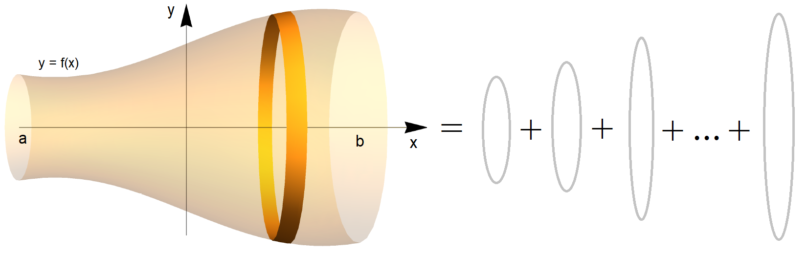
Fig. 10.9 Left Pane: Rotating a function \(y = f(x)\) around the \(x\) axis, over \(x \in [a,\, b]\) producing a solid of revolution, Right Pane: Breaking down the volume into discrete slices, each of width \(\mathrm{d} x\).

To find the volume of such a rotated solid, we need to think about the cross sectional area along the range, which will be \(\pi \,y^2\) since the radius of each slice at \(x\) is \(y(x)\). Then we just need to integrate up these slices \(\pi\,y^2\,\mathrm{d}x\) over the range:

\[V_x = \int_a^b \pi\,y^2\,\mathrm{d}x\]

and we can swap round the axis we rotate over to the \(y\) axis and therefore the radius of each slice would be \(\pi\,x^2\) and therefore:

\[V_y = \int_{y(a)}^{y(b)} \pi\,x^2\,\mathrm{d}y\]

Note

Instead of using cylindrical slices, we could use “frustrums” (sections of cones). The result would be the same (in the limit \(\Delta x \rightarrow 0\)).

Similarly, when calculating the area under the curve, we used rectangles, but we could have used parallelograms.

We can also find the surface area of this solid of revolution, if we rotate over the \(x\) xcis then this surface area is the circumference of each slice \(2\pi\,y\) multiplied by the path length \(\mathrm{d} s\) along the surface, so we find:

\[A_x = \int_{x=a}^{x=b} 2\pi\,y\,\mathrm{d}s = \int_a^b 2\pi\,y\,\sqrt{1 + \left(\frac{\mathrm{d}y}{\mathrm{d}x}\right)^2}\,\mathrm{d}x\]

We could rotate over the \(y\) axis instead, in which case we just switch the circumference we are interested in to be \(2\pi\,x\) and integrate the path length over the \(y\) axis:

\[A_y = \int_{y(a)}^{y(b)} 2\pi\,x\,\mathrm{d}s = \int_{y(a)}^{y(b)} 2\pi\,x\,\sqrt{1 + \left(\frac{\mathrm{d}x}{\mathrm{d}y}\right)^2}\,\mathrm{d}y\]

Worked example

Lets find the volume of a cone depicted in Fig. 10.10, with height \(h\) and circular radius \(R\), so \(y = R x / h\) over the range \(x \in [0,\, h]\):

\[\begin{split}V_x = \int_0^h \pi\,\left(\frac{R x}{h}\right)^2\,\mathrm{d}x = \frac{R^2 \,\pi}{h^2}\Big[ \frac{1}{3}x^3\Big]_0^h = \frac{1}{3}\pi \,R^2\,h\\\end{split}\]

which matches the expression we expect and explains where this factor of \(1/3\) comes from!

Likewise we can look at the surface area of this cone, \(y = R x / h \rightarrow \mathrm{d}y/\mathrm{d}x = R / h\) over the range \(x \in [0,\, h]\):

\[\begin{split}A_x &= \int_0^h 2\pi\,\frac{R x}{h}\,\sqrt{1 + \left(\frac{R}{h}\right)^2}\,\mathrm{d}x \\ &= 2\pi \frac{R}{h}\sqrt{1 + \left(\frac{R}{h}\right)^2}\Bigg[ \frac{1}{2}x^2\Bigg]_0^h \\ &= \pi R h\sqrt{1 + \left(\frac{R}{h}\right)^2} = \pi R\sqrt{h^2 + R^2}\end{split}\]

where \(\sqrt{h^2 + R^2}\) is the slant length.

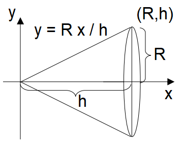
Fig. 10.10 Depiction of a function \(y = R x / h\) and the solid of revolution around the \(x\) axis - a cone.

Likewise if we have parametrised expressions \(x = x(t),\, y = y(t)\), over the range \(t \in [t_1,\, t_2]\) then these expressions become:

\[\begin{split}V_x &= \int_{t_1}^{t_2} \pi\,y^2\,\frac{\mathrm{d}x}{\mathrm{d}t}\,\mathrm{d}t \\ V_y &= \int_{t_1}^{t_2} \pi\,x^2\,\frac{\mathrm{d}y}{\mathrm{d}t}\,\mathrm{d}t \\ A_x &= \int_{t_1}^{t_2} 2\pi\,y\,\sqrt{\left(\frac{\mathrm{d}x}{\mathrm{d}t}\right)^2 + \left(\frac{\mathrm{d}y}{\mathrm{d}t}\right)^2}\,\mathrm{d}t \\ A_y &= \int_{t_1}^{t_2} 2\pi\,x\,\sqrt{\left(\frac{\mathrm{d}x}{\mathrm{d}t}\right)^2 + \left(\frac{\mathrm{d}y}{\mathrm{d}t}\right)^2}\,\mathrm{d}t\end{split}\]

Practice questions

1. Find the surface area of revolution for \(y = x^2\) rotated around the \(y\) axis over \(y \in [0,\,4]\).

2. Determine the surface area of the solid obtained by rotating the function \(y=\sqrt{9-x^2}\) for \(-2 \leq x \leq 2\) about the \(x\)-axis.

3. Determine the surface area of the solid obtained by rotating the function \(y=x^{1/3}\), for \(1 \leq y \leq 2\) about the \(y\)-axis.

4. Find the surface area spherical section obtained by revolving the function \(r = \cos(\theta)\) around the \(x\) axis over \(\theta \in \left[0\,\frac{\pi}{4}\right]\).

5. Find the volume of revolutio for the section obtained by reolving the function \(y = x^2\) around the \(x\) axis over \(x \in [-2,\,3]\).

6. Find the volume of the solid obtained by rotating the region bounded by \(y=2x^2\) and \(y=x^3\) about the \(x\) axis, from the origin up to where the functions meet.

Solution

1.

\[\begin{split}y = x^2\Rightarrow x = y^{1/2}\\ \frac{\mathrm{d}x}{\mathrm{d}y} = \frac{1}{2}y^{-1/2}\\ 1 + (x')^2 = 1 + \frac{1}{4}y^{-1} = \frac{1+4y}{4y}\end{split}\]

so integral is:

\[\begin{split}A &= \int_{y=0}^{y=4} 2\pi\,x\,\mathrm{d}s = 1\pi\int_0^4 x\,(1+4x^2)^{1/2}\,\mathrm{d}x \\ &= \frac{\pi}{4}\bigg[\frac{2}{3} (1+4x^2)^{3/2} \bigg]_0^2 = \frac{\pi}{6}\left(17^{3/2}-1\right) \approx 36.2\dots\end{split}\]

2.

\[\begin{split}y^2 &= 9-x^2\\ 2y\frac{\mathrm{d}y}{\mathrm{d}x} &= -2x \Rightarrow \frac{\mathrm{d}y}{\mathrm{d}x} = -\frac{x}{y} = -\frac{x}{\sqrt{9-x^2}}\\ 1 + \left( \frac{\mathrm{d}y}{\mathrm{d}x}\right)^2 &= 1 + \frac{x}{9-x^2} = \frac{9}{9-x^2}\end{split}\]

so integral is:

\[2\pi\,\int_{-2}^2 y\sqrt{1 + \left( \frac{\mathrm{d}y}{\mathrm{d}x}\right)^2}\,\mathrm{d}x = 6\pi\,\int_{-2}^2 \, \mathrm{d}x = 24\pi\]

3.

\[\begin{split}y &= x^{1/3} \Rightarrow x = y^3\\ \frac{\mathrm{d}x}{\mathrm{d}y} &= 3y^2 \\ 1 + \left( \frac{\mathrm{d}x}{\mathrm{d}y}\right)^2 &= 1+ 9y^4 \end{split}\]

the limits as \(y \in [1,\, 2]\), so integral is:

\[2\pi\,\int_{1}^2 x\sqrt{1 + \left( \frac{\mathrm{d}x}{\mathrm{d}y}\right)^2}\,\mathrm{d}x = 2\pi\int_{1}^2 y^3\left(1+9y^4\right)^{1/2}\, \mathrm{d}x\]

which we can solve by inspection (or reverse chain rule), where \(\int f^n\,f'\,\mathrm{d}y = \frac{1}{n+1}f^{n+1}\), here \(f = 1+9y^4 \), so \(f' = 36y^3\)

\[S = 2\pi\frac{1}{36}\Big[\frac{2}{3}\left(9y^4+1 \right)^{3/2}\Big]_1^2 = \frac{\pi}{27}\left(145^{3/2} - 10^{3/2} \right) \simeq 199.48\dots\]

4. Given that the surface for a rotated solid around the \(x\) axis is \(\int_a^b 2\pi y\,\mathrm{d}s\) and we have \(x = r \cos(\theta),\, y = r \sin(\theta)\), then this is just a parametric problem, where:

\[\begin{split}\mathrm{d}s &= \sqrt{\left(\frac{\mathrm{d}x}{\mathrm{d}\theta}\right)^2 + \left(\frac{\mathrm{d}y}{\mathrm{d}\theta}\right)^2}\,\mathrm{d}\theta\\ \mathrm{d}x &= \cos(\theta)\,\mathrm{d}r - r \sin(\theta)\,\mathrm{d}\theta \Rightarrow \frac{\mathrm{d}x}{\mathrm{d}\theta} = \cos(\theta)\,\frac{\mathrm{d}r}{\mathrm{d}\theta} - r \sin(\theta)\\ \mathrm{d}y &= \sin(\theta)\,\mathrm{d}r + r \cos(\theta)\,\mathrm{d}\theta \Rightarrow \frac{\mathrm{d}y}{\mathrm{d}\theta} = \sin(\theta)\,\frac{\mathrm{d}r}{\mathrm{d}\theta} + r \cos(\theta)\\ \mathrm{d}s &= \sqrt{r^2 + \left(\frac{\mathrm{d}r}{\mathrm{d}\theta}\right)^2}\,\mathrm{d}\theta \end{split}\]

Given that \(r = \cos(\theta)\) then:

\[\frac{\mathrm{d}r}{\mathrm{d}\theta} = -\sin(\theta)\]

so the problem looks like:

\[\begin{split}A &= \int_0^{\pi/4} 2\pi r\,\sin(\theta)\,\sqrt{\cos^2(\theta) + \sin^2(\theta)}\,\mathrm{d}\theta \\ &= \int_0^{\pi/4} 2\pi \cos(\theta)\,\sin(\theta)\,\mathrm{d}\theta = \Bigg[\pi \sin^2(\theta) \Bigg]_0^{\pi/4} = \frac{\pi}{2}\end{split}\]

5.

Using \(V = \int_{-2}^3 \pi y^2\,\mathrm{d}x \), we find:

\[V = \int_{-2}^3 \pi x^4\,\mathrm{d}x = \Bigg[ \frac{1}{5}x^5\Bigg]_{-2}^3 = \pi\left[ \frac{243}{5} - \left(-\frac{32}{5}\right)\right] = 55\pi\]

6.

Firstly lets find the intersection points:

\[\begin{split}x^3 &= 2x^2 \\ x^2(x-2) &= 0 \\ \Rightarrow x = 0,\qquad & x = 2\end{split}\]

which we can also see graphically:

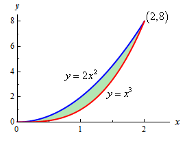
To find the volume of the bounded shape, we need to subtract the two volumes we would find:

\[\begin{split}V_{tot} &= V_{outer} - V_{inner} = \int_0^2 \pi (2x^2)^2 \,\mathrm{d}x - \int_0^2 \pi (x^3)^2 \,\mathrm{d}x \\ &=\int_0^2 \pi \left(4x^4 -x^6\right)\, \mathrm{d}x = \Bigg[ \frac{4}{5}x^5 - \frac{1}{7}x^7\Bigg]_0^2 = \frac{256}{35}\pi\end{split}\]

previous

9. Differentiation

next

11. Multivariable Calculus