Matrices
Contents
7. Matrices
7.1. Matrix Definitions
A matrix (plural: matrices) is essentially just an array of values, arranged in rows and columns.
In general, the values contained in a matrix could represent anything, although manipulating systems of linear equations is one of the most valuable uses of matrices.
7.1.1. Notation
Two example matrices are given below
It is important that you do not use commas to separate the elements, which is incorrect notation.
Either square or round brackets can be used to denote a matrix - but you should avoid mixing notation. Other types of brackets cannot be used, so none of the expressions below are matrices. In fact, the third expression has a special meaning, as we will see later.
7.1.2. Terminology
The matrix featured in (7.1) is referred to as a square matrix because it has the same number of rows and columns. We also can say that it is a (2x2) matrix, because it has two rows and two columns.
The number of rows must be given first:
\( \left( \begin{matrix} 1 & -3 & 5\\ 2 & -1 & 7\end{matrix} \right) \) is a (2 x 3) matrix, whereas \( \left( \begin{matrix} 1 & -3 \\ 2 & -1 \\ 5 & 7\end{matrix} \right) \) is a (3 x 2) matrix.
This measurement is properly referred to as the order of a matrix, but is also often referred to as the size. The individual values in a matrix are called elements, so in the matrix \( M = \left( \begin{matrix} 1 &2 &3 \\ 4& 5& 6\end{matrix} \right) \) we can say that the element in the \(2^{nd}\) row and \(3^{rd}\) column is the number 6. Subscripts can be used to refer to the elements, by writing \( M_{2,3} = 6\) for example.
The transpose of a matrix, written with a superscript letter T, means that we swap the rows and columns,:
In element notation, for any matrix \(X\), we can write that \(\left(X^T\right)_{i,j} = X_{j,i}\). That is, the element in the \(i^{th}\) row and \(j^{th}\) column of \(X\) becomes the element in the \(j^{th}\) row and \(i^{th}\) column of \(X^T\).
The order of a matrix is reversed when it it transposed.
In a square matrix, two diagonals are called the main diagonal (top-left two bottom right), and the anti-diagonal (bottom-left to top-right). Square matrices for which \(A_{i,j}=A_{j,i}\) are called symmetric matrices.
An upper-triangular matrix is a square matrix in which the elements below the main diagonal are all zero, and a lower-triangular matrix is one where the elements above the main diagonal are all zero.
A diagonal matrix is one in which all of the elements are zero apart from those on the main diagonal. These type of matrices are very special, since they have “nice” properties for the purpose of matrix algebra.
Practice Questions
1. What is the order of each of the matrices shown?
\(A=\left(\begin{array}{cc}0 & -1 \\2 & 3 \\-1 & 0 \\\end{array}\right), \quad b=\left(\begin{array}{c}1 \\2 \\3 \\\end{array}\right), \quad c=0\).
2. Given the matrix:
what element is represented by \((X^T)_{2,3}\) ?
3. Which of the following matrices is an upper-triangular matrix?
Solutions
1. Order of \(A = \) (3x2) Order of \(b = \) (3x1) Order of \(c = \) (1x1)
2.
Hence \((X^T)_{2,3} = -4\)
3. Matrix \(A\) is in upper-triangular form.
7.2. Matrix algebra
We will look at how real number algebra, such as addition and multiplication, can be extended to work with matrices. These are entirely human constructs, and you may be easily forgiven for asking why do we do it this way?
However, the best way to appreciate the practicalities is by tackling some problems, and so the definitions will first be introduced without much explanation. From a mathematical perspective, we simply note that the definitions must be consistent and well-determined (unambiguous).
7.2.1. Multiplication by a scalar
Let \(\lambda\) be a scalar (a single number) and \(M\) be a matrix. Then \(\lambda M\) means that every element in matrix \(M\) is multiplied by \(\lambda\). This can be written in element notation as follows:
For example:
7.2.2. Addition
Let \(A\) and \(B\) be two matrices of the same order. Then,
The expression states that to add two matrices, we add together the corresponding elements. This type of operation on two matrices can be referred to as an element-wise operation.
For example:
The element-wise property means that only matrices of the same order can be added, and the expressions below are both meaningless:
Matrix addition can be combined with multiplication by a scalar to add multiples of one matrix to another.
For example:
Practice Questions
Given the matrices:
What will be the result of the following expressions?
\(\left(A+B\right)+C\)
\((C+B)+A\)
\(A-2B+\frac{1}{2}C\)
\(A+D\)
Solutions
1.
2.
3.
4. Cannot add matrices of different orders together.
7.2.3. Matrix multiplication
To multiply two matrices together, their inner dimensions must be the same. That is, to calculate \( \boldsymbol{A}\boldsymbol{B} \), the number of columns in \(\boldsymbol{A}\) must be the same as the number of rows in \(\boldsymbol{B}\). The order of the product matrix is given by the outer dimensions of the two matrices. We can represent this result visually:
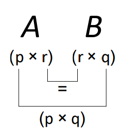
Fig. 7.1 Two matrices A,B can be multiplied if their inner dimensions agree. The dimensions of the result is given by the outer dimensions of AB.
Matrix Multiplication
Given a \((p × r)\) matrix \(\boldsymbol{A}\) and a \((r × q)\) matrix \(\boldsymbol{B}\), the matrix product \(\boldsymbol{A\,B}\) defines a \((p × q)\) matrix, whose elements are given by
To perform matrix multiplication, we must take elements in a row on the left hand side matrix and multiply with elements in a column on the right hand side matrix. The process is illustrate graphically here for a (2 x 2) example:
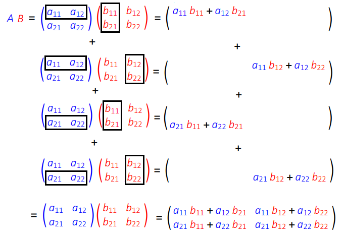
Fig. 7.2 The \((i,\,j)\)th element in the product \(AB\) is given by the product sum of row \(i\) from matrix A with column \(j\) of matrix \(B\).
Practice Questions
Given that
1. Calculate \(AB\) and \(BA\), are these results the same?
2. Explain why the result \(A\left(\begin{array}{c}1\\2\end{array}\right)\) cannot be calculated.
3. What will be the order of the matrix \(A C\)?
4. Calculate the element in the second row and third column of \(AC\)
5. Calculate the result \(D^2\) (this question is a bit boring, but good practice!)
Solutions
1.
Hence \(AB \neq BA\)!
2. The nunber of columns in \(A\) do not match the number of rows in \(\left(\begin{array}{c}1\\2\end{array}\right)\), so it is unclear what to do with the additional numbers in \(A\)!
3. \(AC\) is a \((2 \times 3) \times (3 \times 4) = (2 \times 4)\) matrix.
4. \(A_{2,3} = 4\)
5.
7.2.4. Properties of matrix multiplication
Matrix multiplication is associative, that is:
This can be proved by showing that the left and right hand sides are the same order, and that
Warning
Matrix multiplication is NOT commutative, that is
although \(AB\) and \(BA\) may be equal in some special cases, but not in general!
Worked Example
7.3. The identity matrix
Definition
The identity matrix
We usually drop the subscript \(n\) when working with the identity matrix, because the order can be inferred.
The identity matrix \(I_n\) is the unique \((n \times n)\) matrix which has the property
for any \(x \in \mathbb{R}^n\).
The identity matrix transforms the vector \(x\) to itself. It plays the same role in matrix multiplication as the number 1 does for multiplication of real numbers.
Practice Questions
1. Calculate \(I\begin{pmatrix}1 & 2\\3 & 4\end{pmatrix}\) and \(\begin{pmatrix}1 & 2\\3 & 4\end{pmatrix}I\).
2. Use the identify matrix to factorise
where \(\lambda\) is a scalar and \(A,\,B\) are square matrices.
Solutions
1.
2.
7.4. Matrices and simultaneous equations
We can make the connection between matrices and linear systems of equations, our aim is to find the general solution to the equation:
where \(A\) is an \((m \times n)\) matrix and \(b \in \mathbb{R}^m\) and \(x \in \mathbb{R}^n\) are vectors.
Such an equation is exactly equivalent to a linear system of \(m\) equations in \(n\) unknowns. For example, we can write the system
as the matrix equation
Matrix Equation
The linear system of equations
is equivalent to the matrix equation
where: \(A=\begin{pmatrix} a_{1,1} & \cdots & a_{1,n}\\ \vdots & \ddots & \vdots\\ a_{m,1} & \cdots & a_{m,n} \end{pmatrix}\), \(x=\begin{pmatrix}x_1\\ \vdots \\ x_n\end{pmatrix}\) and \(b=\begin{pmatrix}b_1\\ \vdots \\b_m\end{pmatrix}\)
This equivalence means that we can move freely between these two ways of writing and thinking about a linear system.
7.5. Matrix determinant
The determinant is a single number calculated from a square matrix. The determinant tells us whether the matrix is invertible, as well as a lot of other useful information about the matrix. We find that calcualtign the determinant for (2×2) and (3×3) matrices most useful with a number of direct applications, in this section we will study properties of the determinant and methods for calculating it.
(2x2) Determinant
For a (2x2) matrix, the determinant is given by subtracting the product of the anti-diagonal elements from the product of the leading diagonal elements.
Thus the determinant of a (2x2) matrix \(A\):
is given by:
This is also written as \(\text{det}(A)\) and/or with the notation \(|A|\).
We note that \(\text{det}(A)\) is a scalar quantity.
(3x3) Determinant
For a (3x3) matrix \(A\):
the matrix determinant can be found by finding the determinants of each minor of the matrix \(A\):
This represents just one way to find the minor matrices, we could also pick any other row, column (or even diagonal) and construct the matrix of minors from \(A\) and then find these determinants.
7.5.1. Properties of matrix determinants
Let \(A\) be an \((n \times n)\) matrix:
1. The determinant of the identity matrix is always 1.
2. The determinant reverses sign when any two rows are exchanged.
3. The determinant is a linear function of each of the rows.
4. If one row is equal to another row then \(\det(A)=0\).
5. Adding a multiple of one row to another row leaves \(\det(A)\) unchanged.
6. If \(A\) has a zero row then \(\det(A)=0\).
7. If \(A\) is triangular then \(\det(A)\) is the product of the diagonal elements.
8. \(A\) is invertible if and only if \(\det(A)\neq 0\).
9. \(\det(AB) = \det(A)\det(B)\).
10. \(\det(A^{T}) = \det(A).\)
7.6. Matrix Inverses
Definition
Let \(A\) be an \((n \times n)\) square matrix. If there is an \((n \times n)\) matrix \(B\) such that
then \(A\) is invertible and \(B\) is the inverse of A.
We write \(B = A^{-1}\).
In general, if \(A\) is an \(n \times n\) matrix and \(B\) is its inverse, then \(B\) is also an \((n \times n)\) matrix which satisfies
for all \(x \in \mathbb{R}^n\).
In other words, \(AB\) is a matrix which leaves \(x\) unchanged. The only matrix which leaves \(x\) unchanged is the identity matrix \(I\).
7.6.1. Solving Matrix Equations
Suppose that we are given the definitions below and asked to compute the result for \(B\) :
If this was ordinary scalar algebra, then \(B\) would be given by \(\displaystyle \frac{AB}{A}\), but we have not defined the concept of division for matrices.
Indeed, we should recognise a difficulty in doing so, since matrix multiplication is not commutative. The problems \(Q X = P\) and \(X Q=P\) do not generally have the same solution, and so the expression \(\displaystyle X=\frac{P}{Q}\) would be ambiguous.
This difficulty could be addressed by introducing separate concepts of “left-division” and “right-division”, and some authors have done exactly this. However, a more fundamental approach is to abandon the idea of division for matrices altogether, and consider what it means for matrix multiplication to be invertible. To illustrate the use of the inverse matrix, we multiply each side of the equation for \(A B\) in (7.2) by \(A^{-1}\) as follows:
It is very important to recognise that we must do exactly the same thing to both sides of the equation. Since we pre-multiply (left multiply) the left-hand side by \(A^{-1}\), we must also pre-multiply the right-hand side by \(A^{-1}\). Due to the non-commutative nature of matrix multiplication, the result \(A^{-1}(A B)\) is not the same as the result \((A B)A^{-1}\). Now, since matrix multiplication is associative, the left hand side of (7.3) can be rewritten as \((A^{-1} A)B\), and by the definitions of the inverse and identity matrix, we can write \((A^{-1} A)B=I B=B\) in order to obtain
Thus, the result for \(B\) can be determined by performing a matrix multiplication, provided that we can find \(A^{-1}\).
Solving \(AX=B\) and \(XA=B\)
Let \(A\) be an invertible \((n \times n)\) square matrix and \(B\) an (\(n \times m)\) matrix. Then:
\(A X = B\) has solution \(X=A^{-1}B \)
\(X A = B\) has solution \(X=B A^{-1}\).
Worked example
Given that \(C\, X\, D = E\), write down the solution for \(X\) explicitly in terms of inverse matrices \(C^{-1}\) and \(D^{-1}\).
7.6.2. Calculating the (2x2) inverse matrix
The inverse of a (2x2) matrix
The inverse of a (2x2) matrix \(A=\left(\begin{array}{cc}a_{11} & a_{12} \\a_{21} & a_{22} \end{array}\right)\) is given by
and
\(\text{adj}(A)\) is known as the adjugate matrix. For a (2x2) matrix, the adjugate is given by swapping the diagonal elements and multiplying the anti-diagonal elements by -1.
Practice Questions
1. Calculate the determinant of the matrix \(M=\left(\begin{array}{cc}2 & -1 \\3 & 4 \end{array}\right)\).
2. Write the equations below in the form \(Ax=b\):
Calculate the coefficient matrix \(A\) and hence obtain the solution for \(x\)
Solutions
1.
2.
Calculate the coefficient matrix \(A\) and hence obtain the solution for \(x\)
7.6.3. A derivation of the (2x2) matrix inverse
Consider the problem \(A X = I\), which has solution \(X=A^{-1}\). To see how this arises in the (2x2) case, lets think back to simultaneous equations, trying to solve \(Ax = B\):
which we can write as a matrix equation:
Therefore to solve for \(x = A^{-1}B\) we could just invert the siultaneous equations to find the solutions - in general this is best done with the process of row reduction operations (also called Gaussian elimination), but you will study more on this in future courses.
Taking (7.4) and multiplying between lines to have a common factor in the \(x_1\) term:
and then subtracting:
and doing the same procedure to the \(x_2\) term:
and then subtracting:
where we recognise that \(\det(A) = a_{22}\,a_{11} - a_{12}\,a_{21}\) and therefore rewriting this as a set of matrix equations:
which is indeed the matrix inverse for a \((2x2)\) matrix.
7.6.4. Inverse of the Matrix Product
By associativity of matrix multiplication:
Therefore we can see that:
This result satisfies the “common sense” idea (seen in function composition) that inversion comes in reverse order. If transform \(B\) follows transform \(A\) then we have to reverse transform B before reversing A. We remove the outer operation first.
We can liken the result to the operation of getting dressed/undressed: If you put your socks on before your shoes, you have to take your shoes off before you can remove your socks!