2. Infinite powers

This chapter is about the mathematical concepts of order of magnitude and Taylor series. After working through the chapter you should be able to find Maclaurin and Taylor series expansions for given functions and discuss their convergence using numeric justification

2.1. Order of magnitude

When describing the smallness or bigness of numbers it can be helpful to classify them into powers of a given reference quantity (called the base). Customarily we use base 10, though base 2 is used to describe computer memory, and in advanced mathematics it is common to use a base defined by a property of the system being investigated. We may denote the order of magnitude using the symbol $\mathcal{O}$.

In base 10, the order of magnitude is given by the power in scientific notation. For example, the value $3.124\times {10}^3$ is $\mathcal{O}({10}^3)$.

An order of magnitude estimate keeps only the most significant digit in scientific number format. For instance, an order of magnitude estimate for the number of humans on Earth is $8\times {10}^9$. More precise values can be used in the steps towards working out an order of magnitude estimate.

Two physical quantities are said to be the same order of magnitude if their ratio lies between 1/10 and 10. For instance, the value $6.4\times {10}^4$ and $1.2\times {10}^5$ are the same order of magnitude.

Exercise 2.1

By one estimate there are around $2\times {10}^{16}$ ants on Earth, with an average biomass of 0.62mg.

The world population of humans is around $8\times {10}^9$, with an average mass of 50kg including children, of which around 15% is biomass.

Calculate the total ant biomass and the total human biomass. Are these the same order of magnitude?

Click to show

Expressing the total mass in kg, using the result $1\text{mg}={10}^{-6}\text{kg}$:

• Ant biomass : $1.24\times {10}^{10}$kg

• Human biomass: $6\times {10}^{10}$kg

The ant biomass and human biomass are the same order of magnitude, with a ratio around 21%.

2.2. Asymptotic equivalence

Whereas the limit of a function refers to tendency towards a single value, asymptotic equivalence refers to tendency towards a relationship.

For “very small” $x$, the following expressions are asymptotically equivalent:

(2.1)$$\begin{array}{r}\begin{array}{rlrlrlrl}& (1+x{)}^k& & \sim 1& & +kx& & +\frac{1}{2}k(k-1)x^2+\frac{1}{3!}k(k-1)(k-2)x^3+\mathcal{O}(x^4)\\ & e^x& & \sim 1& & +x& & +\frac{x^2}{2}+\frac{x^3}{3}+\mathcal{O}(x^4)\\ & \sin (x)& & \sim x& & -\frac{x^3}{3!}& & +\frac{x^5}{5!}-\frac{x^7}{7!}+\mathcal{O}(x^9)\\ & \cos (x)& & \sim 1& & -\frac{x^2}{2!}& & +\frac{x^4}{4!}-\frac{x^6}{6!}+\mathcal{O}(x^8)\\ & \ln (1+x)& & \sim x& & -\frac{x^2}{2}& & +\frac{x^3}{3}-\frac{x^4}{4}+\mathcal{O}(x^5)\end{array}\end{array}$$

Notice that if $x\ll 1$ (“much less than one”) the higher powers are successively smaller. For instance, if $x=0.1$ the $x^3=0.001$. Therefore the leading terms are most significant in the expansion and the higher powers are “corrections”. In most practical applications we only need the first two or three terms as the rest of the terms can be neglected.

By way of example, consider the plots below, which show the curve $y=e^x$ together with its linear, quadratic and cubic asymptotic expansions.

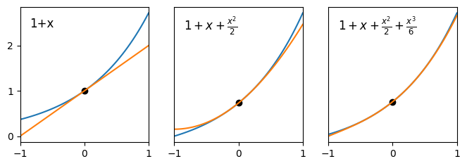
Fig. 2.1 Comparison of asymptotic expansions to the curve $y=e^x$ on the domain $[-1,1]$.

We see that the linear approximation is an accurate representation of the curve in a very small domain close to $x=0$, and that by adding the quadratic and cubic terms we successively improve the approximation on the domain $[-1,1]$.

2.3. Power series construction

To construct expansions of this type, we suppose that we can express a given function $f(x)$ as a sum of the form

(2.2)$$p(x)=c_0+c_{1}x+c_2{x}^2+\cdots +c_n{x}^n+\mathcal{O}(x^{n+1}).$$

The coefficients $c_{0\dots n}$ will be chosen to give an accurate representation of $f(x)$ in the neighbourhood of $x=0$.

Exercise 2.2

Find the first three derivatives of $p(x)$ and evaluate them at $x=0$.

Click to show

$\begin{array}{rlrlrlrlrl}{p}^{\prime }(x)& =c_1& +& 2c_{2}x& +& 3c_3{x}^2& +\dots & +n{c}_n{x}^{n-1}& & +\mathcal{O}(x^n)\\ p^{\prime \prime }(x)& =& & 2c_2& +& 6c_{3}x& +\dots & +n(n-1)c_n{x}^{n-2}& & +\mathcal{O}(x^{n-1})\\ p^{\prime \prime \prime }(x)& =& & & & 6c_3& +\dots & +n(n-1)(n-2)c_n{x}^{n-3}& & +\mathcal{O}(x^{n-2})\end{array}$

$p(0)=c_0,p^{\prime }(0)=c_1,p^{\prime \prime }(0)=2c_2,p^{\prime \prime \prime }(0)=6c_3$

---

Exercise 2.3

Determine a general result for the $n$th derivative $p^{(n)}(0)$.

Match this to $f^{(n)}(0)$ to find an expression for $c_n$.

Click to show

$p^{(n)}(x)=n!c_n+\mathcal{O}(x)⟹p^{(n)}(0)=n!c_n$

Assuming this matches $f^{(n)}(0)$ gives $c_n=\frac{f^{(n)}(0)}{n!}$

Note: $n!=n(n-1)(n-2)\dots 1$
(e.g. $6!=3\times 2=6$)

---

Exercise 2.4

Calculate the first three non-zero terms in the expansion for $f(x)=\ln (1+x)$, using the formula for the coefficients found in the previous exercise.

Click to show

$n$	$f^{(n)}(x)$	$f^{(n)}(0)$	$c_n$
$0$	$\ln (1+x)$	$0$	$0/0!=0$
$1$	$(1+x{)}^{-1}$	$1$	$1/1!=1$
$2$	$-(1+x{)}^{-2}$	$-1$	$-1/2!=1/2$
$3$	$2(1+x{)}^{-3}$	$2$	$2/3!=1/3$

The expansion is

$$p(x)=x-\frac{x^2}{2}+\frac{x^3}{3}+\mathcal{O}(x^4)$$

We can plot this together with $\ln (1+x)$ on the range [-1,1]. The representation is faithful close to $x=0$, but gets worse away from this point, particularly in the negative $x$-direction.

import numpy as np
import matplotlib.pyplot as plt

x=np.linspace(-1,1)
y=np.log(1+x)

plt.plot(x,y,label=r'$\ln(1+x)$')
p=x-x**2/2+x**3/3
plt.plot(x,p,label='$p(x)$')
plt.legend()
plt.show()

---

2.4. Convergence

In the above discussion we assumed that $|x|<1$ so that the powers of $x$ grow successively smaller. However, it is not guaranteed that the infinite sum $p(x)$ will converge to $f(x)$ on the whole interval $[-1,1]$. By constructing the expansion to match the derivatives of $f(x)$ at $x=0$ we have only ensured that the representation is accurate in some local neighbourhood of this point.

It is possible to use tools of mathematical analysis to formally determine the interval of convergence for the infinite series, which will be different for each function $f(x)$. In the case of the series for $\ln (1+x)$ it turns out that the infinite series converges to the correct value on the whole interval $[-1,1]$, albeit rather slowly for some values of $x$.

What is truly remarkable is that for some functions the expansions constructed by the method outlined above are valid over a wider interval than $[-1,1]$. In fact, the expansions for some functions are valid for all values of $x$. Examples include the functions $e^x$, $\sin (x)$ and $\cos (x)$.

It is quite exciting to think that these non-polynomial functions can be represented by infinite polynomial series. However, the expansions converge increasingly slowly as we move further from the point $x=0$, which lessens their practical use.

Here we will not develop the tools of analysis required to undertake a formal investigation of convergence. We will adopt a more experimental approach, by generating series containing a few terms and evaluating their accuracy on the interval that we are interested in.

Exercise 2.5

Demonstrate that with only five terms in the expansion of $\ln (1+x)$ we obtain a result that is accurate to within 1% on the interval $[-0.5,0.5]$

Optional: How many terms are needed in the expansion to obtain a result that is accurate to within 1% on the interval $[-0.99,0.99]$ ?

Click to show

import numpy as np
x=np.linspace(-0.5,0.5,1000)
y=np.log(1+x)

p=x-x**2/2+x**3/3-x**4/4+x**5/5

#maximum relative error
m=max(np.abs((y-p)/y))

#percentage error
print(100*m)

0.6644352054578373

The maximum relative error is 0.664%

To obtain an expansion that is accurate to within 1% on the interval $[-0.99,0.99]$ requires 203 terms. For practical purposes, we normally want to use expansions with only a few terms.

---

2.5. Generalization

In the outline above we developed a power series expansion technique that was accurate in the neighbourhood of $x=0$. For some series derived in this way the results can converge to the correct value on an extended interval. However, even where this is the case we normally require a large number of terms to be kept to obtain a good approximation away from the origin.

Where we require a power series approximation to a function near to a non-zero location, a better technique is to construct the expansion so that it has greatest accuracy in the neighbourhood of the point of interest. We do this using a shifted version of the expansion formula:

(2.3)$$p(x;a)=c_0+c_1(x-a)+c_2(x-a{)}^2+\cdots +c_n(x-a{)}^n+\mathcal{O}((x-a{)}^{n+1})$$

By applying the technique of matching derivatives at $x=a$, we obtain the result

(2.4)$$c_n=\frac{f^{(n)}(a)}{n!}.$$

The formula (2.3) together with (2.4) is known as Taylor’s series. The special case when $a=0$ is known as the Maclaurin series for historical reasons.

Exercise 2.6

Find the first four non-zero terms of the Taylor series for the following cases:

• $e^x$ about the point $x=1$

• $\sin (x)$ about the point $x=\pi /3$

Click to show

$n$	$f^{(n)}(x)$	$f^{(n)}(1)$	$c_n$
$0$	$e^x$	$e$	$e/0!=e$
$1$	$e^x$	$e$	$e/1!=e$
$2$	$e^x$	$e$	$e/2!=e/2$
$3$	$e^x$	$e$	$e/3!=e/6$

Hence $p(x;e)\sim e(1+x+x^2/2+x^3/6+\dots )$

The result could have been obtained by recognising that

$$e^{1+x}=e^1{e}^x$$

and obtaining the expansion for $e^x$ about $x=0$.

Click to show

$n$	$f^{(n)}(x)$	$f^{(n)}(\pi /3)$	$c_n$
$0$	$\sin (x)$	$\sqrt{3}/2$	$\sqrt{3}/2/0!=\sqrt{3}/2$
$1$	$\cos (x)$	$1/2$	$1/2/1!=1/2$
$2$	$-\sin (x)$	$-\sqrt{3}/2$	$-\sqrt{3}/2/2!=\sqrt{3}/4$
$3$	$-\cos (x)$	$-1/2$	$-1/2/3!=-1/12$

Hence

$$p(x;\frac{\pi }{3})\sim \frac{\sqrt{3}}{2}+\frac{x}{2}-\frac{\sqrt{3}}{4}{x}^2-\frac{x^3}{12}$$

Exercise 2.7

Explain why it is not possible to construct a series expansion of $\ln (x)$ about the point $x=0$.

Also explain the relationship between the series for $\ln (1+x)$ about $x=0$ and the series for $\ln (x)$ about $x=1$.

Click to show

The function $\ln (x)$ is not defined at $x=0$.

The series for $\ln (x)$ about $x=1$ is identical to the series for $\ln (1+x)$ about $x=0$.

This can be seen by defining $\hat{x}=x-1$.

2.6. Order of accuracy

We assume the Taylor series is to be used in the neighbourhood of the expansion point, so $(x-a)$ is a small quantity. We say that the degree $n$ series has “order $(x-a{)}^n$ accuracy” and we may write

(2.5)$$f(x)=p_n(x;a)+\mathcal{O}((x-a{)}^{n+1}),$$

where the “big-O” notation describes the size of the error terms.

This finding can be used to describe the size of the error in the finite difference approximation presented in the last chapter. Discarding all terms of degree greater than one in Taylor’s expansion about $x=x_k$ gives:

(2.6)$$y(x)=y(x_k)+y^{\prime }(x_k)(x-x_k)+\mathcal{O}((x-x_k{)}^2)$$

If we label $h=(x-x_k)$, then we may rewrite the expression as shown below. The result is known as Euler’s forward difference formula or the explicit Euler method.

(2.7)$$y(x_k+h)=y(x_k)+y^{\prime }(x_k)h+\mathcal{O}(h^2),h\ll 1$$

A simple rearrangement of Euler’s forward difference formula gives the previously obtained expression for the derivative at $x_k$

(2.8)$$y^{\prime }(x_k)=\frac{y(x_k+h)-y(x_k)}{h}+\mathcal{O}(h).$$

The result also shows that the error in this expression is order $h$, as discovered when we plotted the error against the step size. The error is due to working with finite approximations to infinitesimal quantities, and is a result of truncating the Taylor expansion after just two terms.

We should distinguish truncation error from the previously seen roundoff errors that occur as a computational artefact due to working with finite precision arithmetic.

Warning

A proper mathematical description of the order of magnitude requires the Lagrange remainder theorem, which places an upper bound on the size of the error. The error in the truncated expansion is found to be proportional to the next power of that was discarded in the expansion.