Chapter 8 exercise

The equation can be written out using the central differences formula as:

\[\begin{equation*} \frac{\phi_{i-1}-2\phi_i+\phi_{i+1}}{h^2}+\frac{1}{r_i}\frac{\phi_{i+1}-\phi_{i-1}}{2h}=0 \end{equation*}\]

which rearranges to

\[\begin{equation*} \phi_i=\frac{\left(r_i-\frac{h}{2}\right)\phi_{i-1}+\left(r_i+\frac{h}{2}\right)\phi_{i+1}}{2r_i} \end{equation*}\]

This can be applied as follows

import numpy as np
import matplotlib.pyplot as plt

n=51;                          #We are using 51 points
r = np.linspace(0.05,0.10,n)   #Construct the radial coordinate
h =r[2]-r[1]                     

#Set up the initial grid :
F0 = 400*np.ones(n)       # The temp avg is a suitable choice
F0[0]=500; F0[-1]=300     # Enforce boundary conditions

F1 = np.zeros(F0.shape)   #Initialize

tol=1e-4                  #Error tolerance
err=1                     #Initialise
n=0
while err>tol:
  F1[:]=F0[:]                  #Make an array copy
  n+=1
  for i in range(1,len(F1)-1):
    F1[i] = ((r[i]-h/2)*F1[i-1]+(r[i]+h/2)*F1[i+1])/2/r[i]; 
  err = np.linalg.norm(F1-F0)  #Error
  F0[:]=F1[:]                  #Re-initialise

print('converged after',n, 'iterations')
# Plot and compare to the analytic solution

a=-200/np.log(2); b=500-200*np.log(20)/np.log(2);
Fanalytic= a*np.log(r)+b;

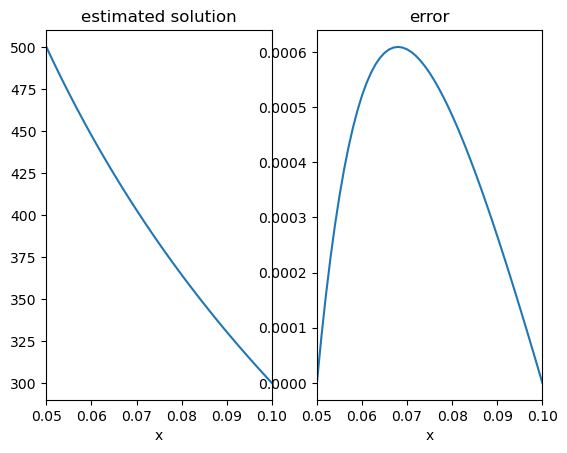
fig,ax = plt.subplots(1,2)
ax[0].plot(r,F1)
ax[0].set_title('estimated solution')
ax[1].plot(r,np.abs(F1-Fanalytic))
ax[1].set_title('error')

ax[0].set_xlim([0.05,0.1])
ax[0].set_xlabel('x')
ax[1].set_xlim([0.05,0.1])
ax[1].set_xlabel('x')

plt.show()

converged after 2204 iterations

At such small step sizes it is the tolerance that dictates the size of the error rather than the step size. Try decreasing the tolerance to 1e-8 and observe the effect on the error.

Also observe that as the step size is decreased, many more iterations are required for the solution to converge.

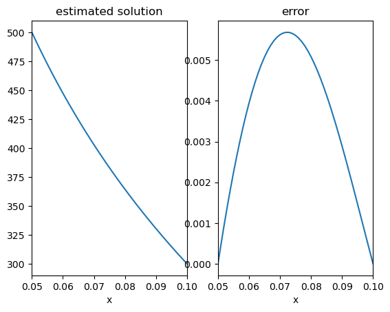
With an over-relaxation parameter of g=1.88 the solution requires 246 iterations to converge to within a tolerance of 1e-8. This is about 20 times less than with no relaxation (g=1).

import numpy as np
import matplotlib.pyplot as plt

n=51;                          #We are using 51 points
r = np.linspace(0.05,0.10,n)   #Construct the radial coordinate
h =r[2]-r[1]                     

#Set up the initial grid :
F0 = 400*np.ones(n)       # The temp avg is a suitable choice
F0[0]=500; F0[-1]=300     # Enforce boundary conditions

F1 = np.zeros(F0.shape)   #Initialize

tol=1e-8                  #Error tolerance
err=1                     #Initialise
g=1.88                    #over-relaxation
n=0
while err>tol:
  F1[:]=F0[:]                  #Make an array copy
  n+=1
  for i in range(1,len(F1)-1):
    F1i = ((r[i]-h/2)*F1[i-1]+(r[i]+h/2)*F1[i+1])/2/r[i];
    F1[i] = F1[i] + g*(F1i-F1[i])  #Relaxation
  err = np.linalg.norm(F1-F0)      #Error
  F0[:]=F1[:]                      #Re-initialise

print('converged after',n, 'iterations')
# Plot and compare to the analytic solution

a=-200/np.log(2); b=500-200*np.log(20)/np.log(2);
Fanalytic= a*np.log(r)+b;

fig,ax = plt.subplots(1,2)
ax[0].plot(r,F1)
ax[0].set_title('estimated solution')
ax[1].plot(r,np.abs(F1-Fanalytic))
ax[1].set_title('error')

ax[0].set_xlim([0.05,0.1])
ax[0].set_xlabel('x')
ax[1].set_xlim([0.05,0.1])
ax[1].set_xlabel('x')

plt.show()

converged after 244 iterations