Chapter 6 exercise

By applying the central formulae (3.6) and (3.3) to replace the first and second derivatives we obtain

(8)\[x_{k+1} = \frac{x_k(2-10h^2)+x_{k-1}(-1+h)}{1+h}\]

Again, we require two starting points. It is tempting to use the explicit Euler method with the first derivative condition to estimate \(x_1\). However, that method is only first order accurate, so this will contaminate our second order accurate algorithm and produce a result that is only \(\mathcal{O}(h)\) accurate.

We therefore use the \(\mathcal{O}(h^2)\) central differences formula for the boundary condition, which gives:

(9)\[\frac{x_1-x_{-1}}{2h} = x^{\prime}_0 \quad \Rightarrow \quad x_{-1}= x_1+2h.\]

This relationship involves the solution at the “ghost” point \(x_{-1}\) where \(t=-h\). We do not know the result at this point, but we can solve the problems for \(x_{-1},x_0,x_1\) simultaneously to obtain our starting points.

From (8) we obtain

\[\begin{equation*} (1+h)x_1 = (2-10h^2)x_0 +(-1+h)x_{-1} \end{equation*}\]

Substituting for \(x_{-1}\) from (9) and using the boundary condition \(x_0=1\) then gives

\[\begin{align*} (1+h)x_1&=(2-10h^2)+(-1+h)(x_1+2h) \\ &\implies x_{-1}=1-h-4h^2. \end{align*}\]

from numpy import arange,cos,exp
import matplotlib.pyplot as plt
plt.rcParams['axes.xmargin'] = 0
h=0.01
t=np.arange(0,10,h)
xsol=exp(-t)*cos(3*t)

n=len(t); x=np.empty(n)   # Pre-allocate
x[0]=1;                   # Initial value
x[1]=1-h-4*h**2           # Ghost point

# Central difference rule
for k in range(1,n-1):
  x[k+1]=((2-10*h**2)*x[k]+(-1+h)*x[k-1])/(1+h)

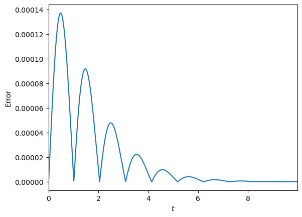
# Compare to analytic solution
plt.plot(t,abs(x-xsol))
plt.xlabel('$t$'); plt.ylabel('Error')
plt.show()