Chapter 1 exercise

Question

The logistic function is given by the following expression in which parameters \(t_0\), \(C\), \(r\) are constants determining the location, scale and shape of the curve:

(1)\[\begin{equation} x=\frac{C}{1+e^{-r(t-t_0)}}. \end{equation}\]

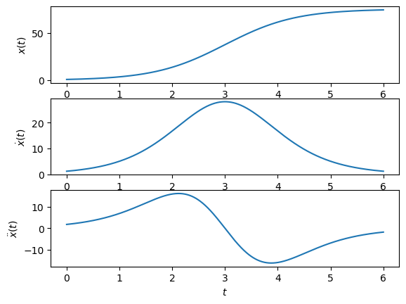
Produce a plot of the function using a step size h=1e-3 for the case where \(t_0=3\), \(C=75\), \(r=1.5\), Use the difference formula to estimate the first and second derivatives numerically.

Solution

Each time we apply the finite difference formula to differentiate, we lose one data point. The question didn’t specify that the three plots must have the same number of datapoints, but here is an example implementation in which all three plots use the same gridpoints:

# Given parameters
t0,r,C = 3,1.5,75
h=1e-3

# Extend interval by two points
t = np.arange(0,6+3*h,h)
x = C/(1+np.exp(-r*(t-t0)))

# Apply difference formula
from numpy import diff
xd = diff(x)/h
xdd= diff(xd)/h

# Make all arrays the same length
t,x = t[0:-2],x[0:-2]
xd  = xd[0:-1]

fig, ax = plt.subplots(3,1)
ax[0].plot(t,x)
ax[0].set_ylabel('$x(t)$')
ax[1].plot(t,xd)
ax[1].set_xlabel('$t$')
ax[1].set_ylabel('$\dot{x}(t)$')
ax[2].plot(t,xdd)
ax[2].set_xlabel('$t$')
ax[2].set_ylabel('$\ddot{x}(t)$')

plt.show()