Chapter 3 exercise
Contents
Chapter 3 exercise#
Question#
The logistic function is given by the following expression in which parameters \(t_0\), \(C\), \(r\) are constants determining the location, scale and shape of the curve:
Taking a step size h=1e-3 and with paramater values \(t_0=3\), \(C=75\), \(r=1.5\), numerically estimate the second derivative of the logistic function:
(a) using the forward difference formula,
(b) using the central difference formula.
You will need to extend the function estimate at two exterior points to obtain a result for the derivative at each point in the interval.
Plot the error in each of your estimates, given that the analytic result satisfies the equation below, and write a short explanation of your findings.
Note
Forward :
Central :
Solution#
There are countless ways of doing this, including loop-based methods. The following implementation is relatively concise and efficient:
t0=3; C=75; r=1.5; tmin=0; tmax=6; h=1e-3
t = np.arange(tmin-h,tmax+3*h,h) #Extend by +2RHS, +1LHS
x = C/(1+np.exp(-r*(t-t0))) #Logistic function
xdd = (x[0:-2]-2*x[1:-1]+x[2:])/h**2 #2nd derivative formula
t,x=t[1:-2],x[1:-2]; #Drop extra gridpoints
xpp = r**2*x*(C-x)*(C-2*x)/C**2 #Analytic result
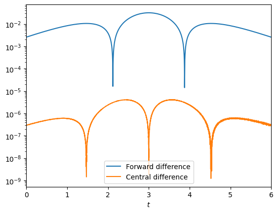
plt.semilogy(t,np.abs(xdd[1:]-xpp) ,label='Forward difference')
plt.semilogy(t,np.abs(xdd[0:-1]-xpp),label='Central difference')
plt.xlabel('$t$'); plt.xlim(tmin,tmax); plt.legend()
plt.show()
Things to look for in solution:
Correct grid spacing as specified by the step size
h=1e-3given in the question. The solution domain should be clearly defined.Correct calculation of the logistic function, with no misplaced brackets!
Accurate implementation of the second derivative formula. Whilst this can be done with a loop-based method, the slicing technique was demonstrated in the notes and such tehniques will form the basis for the extension work on this topic.
The forward and central difference second derivative formulas are identical, but offset by one gridpoint. Solutions that can make use of this demonstrate most sophistication.
The analytic result should be calculated from the given expression involving x. When determining the error it is not essential that the absolute value is taken.
Both error curves should be visible on the solution plot. Here this has been achived using a logarithic scale, but an approach that uses subplots is also acceptable. The plots should be clearly labelled, or at least identifiable.
Ideally, implementations should be concise, clear and efficient. However, the most efficient approach will not necessarily be the clearest! A judgement may need to be made about where to compromise, but answers that are repetitious are generally not the best.
The comment should note that the size of the errors is predicted by the truncation order of the finite difference formulae. In the forward difference formula the error is \(\mathcal{O}(h)\) and in the central difference formula it is \(\mathcal{O}(h^2)\). The solutions we found are broadly consistent with this prediction.