41. Solutions

import numpy as np
import matplotlib.pyplot as plt
import matplotlib.cm as cm

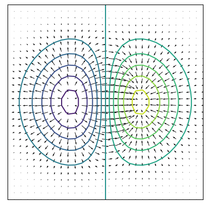
41.1. Chapter exercises 26

The velocity field is given by

\[\begin{equation*} (u,v)=(\phi_x,\phi_y) = (1-2x^2,-2xy)e^{-x^2-y^2} \end{equation*}\]

A plot of the vector field and contours of the potential function is shown below. The contours of the scalar potential are perpendicular to the vector field.

x=np.linspace(-2, 2, 30)
y=np.linspace(-2, 2, 30)

X,Y = np.meshgrid(x, y)  
(U,V)=(1-2*X**2,-2*X*Y)*np.exp(-X**2-Y**2)

# options to prettify the plot
fig,ax=plt.subplots(figsize=(5,5))
ax.axis([-2,2,-2,2])
ax.xaxis.set_ticks([]), ax.yaxis.set_ticks([])

ax.quiver(X,Y,U,V)

ax.contour(X,Y,X*np.exp(-X**2-Y**2),levels=10)

plt.show()

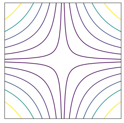
41.2. Chapter exercises 27

Question 1

The streamline for this problem that passes through satisfy \((x_0,y_0)\) at time \(t\) is given as follows:

\[\begin{equation*}\frac{\mathrm{d}x}{\mathrm{d}s}=2x, \quad \frac{\mathrm{d}y}{\mathrm{d}s}=2ts \quad \rightarrow \quad (x,y)=(x_0 e^{2s},y_0 e^{2ts}).\end{equation*}\]

Note that the streamlines satisfy \(y=kx e^{t}\), where \(k=y_0/x_0\).

Question 2

\(\underline{u}=(x^2y,-xy^2)=\left(\frac{\partial\psi}{\partial y},-\frac{\partial\psi}{\partial x}\right) \quad \rightarrow \psi = \frac{x^2 y^2}{2}\)

x=np.linspace(-2, 2, 100)
y=np.linspace(-2, 2, 100)

X,Y = np.meshgrid(x, y)
F=(X**2)*(Y**2)/2

# options to prettify the plot
fig,ax=plt.subplots(figsize=(5,5))
ax.axis([-2,2,-2,2])
ax.xaxis.set_ticks([]), ax.yaxis.set_ticks([])

ax.contour(X,Y,F,levels=[0.005,0.1,0.4,1,2,4])

plt.show()

Question 3

Streamlines :

\(\frac{\mathrm{d}x}{\mathrm{d}s}=\alpha \quad \rightarrow \quad x=\alpha s + x_0\)

\(\frac{\mathrm{d}y}{\mathrm{d}s}=\beta t \quad \rightarrow \quad y=\beta t s + y_0\)

Combining the two expressions gives \(y=\frac{\beta t}{\alpha}(x-x_0)+y_0\). This is the equation of the streamline at time \(t\) that passes through \((x_0,y_0)\).

Particle paths :

\(\frac{\mathrm{d}x}{\mathrm{d}t}=\alpha \quad \rightarrow \quad x=\alpha t +x_0\)

\(\frac{\mathrm{d}y}{\mathrm{d}t}=\beta t \quad \rightarrow \quad y=\beta \frac{t^2}{2}+y_0\)

Combining the two expressions gives \(y=\frac{\beta}{2 \alpha^2}(x-x_0)^2+y_0\). This is the path of a particle released from \((x_0,y_0)\) at time \(t=0\).

For this example, the streamlines are straight lines, and the particle paths are parabolas.

Note

In the case of the streamlines, we may obtain the following result using the chain rule

\(\frac{\mathrm{d}y}{\mathrm{d}x}=\frac{\beta t}{\alpha} \quad \Rightarrow \quad y=\frac{\beta t}{\alpha}x+c\)

However, we cannot use this treatment to solve for the particle paths since in that case \(x=x(t)\), \(y=y(t)\) and so \(t\) must not be treated as constant.

41.3. Chapter exercises 28

Question 1

\(\nabla.\underline{u}=\nabla^2\phi=\frac{\partial^2\phi}{\partial x^2}+\frac{\partial^2\phi}{\partial y^2}=4x(x^2+y^2-2)e^{-x^2-y^2}\)

x=np.linspace(-2, 2, 100)
y=np.linspace(-2, 2, 100)

X,Y = np.meshgrid(x, y)
Z=4*X*(X**2+Y**2-2)*np.exp(-X**2-Y**2)

# options to prettify the plot
fig,ax=plt.subplots(figsize=(5,5))
ax.axis([-2,2,-2,2])
ax.xaxis.set_ticks([]), ax.yaxis.set_ticks([])

# The "pcolormesh" function can be used to make a density plot.
ax.pcolormesh(X,Y,Z,shading='auto',cmap=cm.gray)
plt.show()

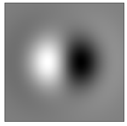
Note: This picture matches with what we found in Chapter exercises 26. From the plot of the vector field we could imply that there is a source in the left half plane and a sink in the right half plane.

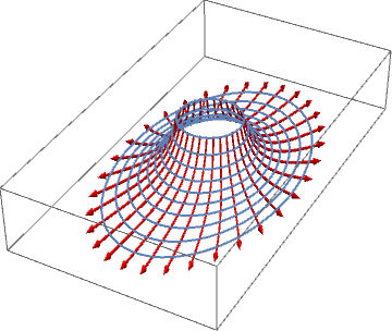
Question 2

Particle paths:

\(\frac{\mathrm{d}x}{\mathrm{d}t}=2x, \quad \frac{\mathrm{d}y}{\mathrm{d}t}=3y, \quad \frac{\mathrm{d}z}{\mathrm{d}t}=-5z\)

Solution: \(x=x_0e^{2t}, \quad y=y_0e^{3t}, \quad z=z_0e^{-5t}\).

Fluid particles that initially lie on the ring \(x_0=\cos(\theta)\), \(y_0=\sin(\theta)\), \(z_0=1\) are described in parametric form by

\(x=\cos(\theta)e^{2t}, \quad y=\sin(\theta)e^{3t}, \quad z=e^{-5t}\)

The equations can also be written as

\(\left(\frac{x}{e^{2t}}\right)^2+\left(\frac{y}{e^{3t}}\right)^2=1, \quad z=e^{-5t}.\)

The equations describe an ellipse parallel to the \((x,y)\) plane at height \(z=e^{-5t}\). The ellipse has major axis \(e^{3t}\) parallel to \(x\) and minor axis \(e^{2t}\) parallel to \(y\).

Particles that initially lie on the ring are therefore swept towards the \((x,y)\) plane and away from the \(z\) axis. This type of motion is called a straining motion.

Irrotational: \(\nabla\times\underline{u}=\begin{vmatrix}\underline{e}_x & \underline{e}_y & \underline{e}_z\\\frac{\partial}{\partial x} & \frac{\partial}{\partial y}& \frac{\partial}{\partial z}\\ 2x & 3y & -5z\end{vmatrix}=0\underline{e}_x+0\underline{e}_y+0\underline{e}_z\)

Solenoidal: \(\nabla.\underline{u} = \frac{\partial}{\partial x}\left(2x\right)+\frac{\partial}{\partial y}\left(3y\right)+\frac{\partial}{\partial z}\left(-5z\right)=0\)

41.4. Chapter exercises 29

Question 1

a). \(\frac{\partial \rho }{\partial t}+u\frac{\partial \rho}{\partial x}+v\frac{\partial \rho}{\partial y}+w\frac{\partial \rho}{\partial z}+\rho \left(\frac{\partial u}{\partial x}+\frac{\partial v}{\partial y}+\frac{\partial w}{\partial z}\right)=0\)

b). Laplace’s equation, \(\nabla^2\phi=0\), where \(\underline{u}=\nabla\phi\)

c). The condition for both types of flow is the same. Since incompressible flows must satisfy \(\nabla.\underline{u}\), they are solenoidal. However, it may be possible for a compressible fluid to exhibit solenoidal flow.

Question 2

(41.1)\[\begin{align} \frac{\partial u}{\partial t}+u\frac{\partial u}{\partial x}+v\frac{\partial u}{\partial y}+w\frac{\partial u}{\partial z}&=-\frac{1}{\rho}\frac{\partial p}{\partial x}\\ \frac{\partial v}{\partial t}+u\frac{\partial v}{\partial x}+v\frac{\partial v}{\partial y}+w\frac{\partial v}{\partial z}&=-\frac{1}{\rho}\frac{\partial p}{\partial y}\\ \frac{\partial w}{\partial t}+u\frac{\partial w}{\partial x}+v\frac{\partial w}{\partial y}+w\frac{\partial w}{\partial z}&=-\frac{1}{\rho}\frac{\partial p}{\partial z}-g\end{align}\]

41.5. Chapter exercises 30

Question 2

(41.2)\[\begin{align} \frac{\partial u}{\partial t}+u\frac{\partial u}{\partial x}+v\frac{\partial u}{\partial y}+w\frac{\partial u}{\partial z}&=-\frac{1}{\rho}\frac{\partial p}{\partial x}+\nu\left(\frac{\partial^2 u}{\partial x^2}+\frac{\partial^2 u}{\partial y^2}+\frac{\partial^2 u}{\partial z^2}\right)\\ \frac{\partial v}{\partial t}+u\frac{\partial v}{\partial x}+v\frac{\partial v}{\partial y}+w\frac{\partial v}{\partial z}&=-\frac{1}{\rho}\frac{\partial p}{\partial y}+\nu\left(\frac{\partial^2 v}{\partial x^2}+\frac{\partial^2 v}{\partial y^2}+\frac{\partial^2 v}{\partial z^2}\right)\\ \frac{\partial w}{\partial t}+u\frac{\partial w}{\partial x}+v\frac{\partial w}{\partial y}+w\frac{\partial w}{\partial z}&=-\frac{1}{\rho}\frac{\partial p}{\partial z}+\nu\left(\frac{\partial^2 w}{\partial x^2}+\frac{\partial^2 w}{\partial y^2}+\frac{\partial^2 w}{\partial z^2}\right)\\ \frac{\partial u}{\partial x}+\frac{\partial v}{\partial y}+\frac{\partial w}{\partial z}&=0\end{align}\]

41.6. Chapter exercises 31

\[\begin{equation*}\frac{\partial u}{\partial x}+\frac{\partial v}{\partial y}=0\end{equation*}\]

Conservation of momentum :

\[\begin{align*} u\frac{\partial u}{\partial x}+v\frac{\partial u}{\partial y}&=-\frac{1}{\rho}\frac{\partial p}{\partial x}+\nu\left(\frac{\partial^2 u}{\partial x^2}+\frac{\partial^2 u}{\partial y^2}\right)\\ u\frac{\partial v}{\partial x}+v\frac{\partial v}{\partial y}&=-\frac{1}{\rho}\frac{\partial p}{\partial y}+\nu\left(\frac{\partial^2 v}{\partial x^2}+\frac{\partial^2 v}{\partial y^2}\right)\\ \end{align*}\]

In terms of the non-dimensional variables (and with the pressure term dropped):

\[\begin{align*}&\frac{U_0^2}{L}\frac{\partial \hat{u}}{\partial\hat{x}}+\frac{V_0}{\delta}U_0\frac{\partial \hat{u}}{\partial\hat{y}}=\nu\left(\frac{U_0}{L^2}\frac{\partial^2 \hat{u}}{\partial\hat{x}^2}+\frac{U_0}{\delta^2}\frac{\partial^2 \hat{u}}{\partial\hat{y}^2}\right)\\ &\Rightarrow \quad \frac{U_0^2}{L}\left[\frac{\partial\hat{u}}{\partial\hat{x}}+\frac{\partial\hat{u}}{\partial\hat{y}}-\frac{\nu}{U_0 L}\left(\frac{\partial^2\hat{u}}{\partial\hat{x}^2}+\left(\frac{L}{\delta}\right)^2\frac{\partial^2\hat{u}}{\partial\hat{y}^2}\right)\right]=0 \end{align*}\]

That is,

\[\begin{equation*} \frac{\partial \hat{u}}{\partial \hat{x}}+\frac{\partial \hat{u}}{\partial \hat{y}}-\frac{1}{R}\left[\frac{\partial^2 \hat{u}}{\partial \hat{x}^2}+\left(\frac{L}{\delta}\right)^2\frac{\partial^2\hat{u}}{\partial \hat{y}^2}\right], \quad R=\frac{U_{\infty} L}{\nu}. \end{equation*}\]

The inertial terms are \(\displaystyle \frac{\partial\hat{u}}{\partial\hat{x}}+\frac{\partial\hat{u}}{\partial\hat{y}}\)

The convective terms are \(\displaystyle \frac{1}{R}\left[\frac{\partial^2\hat{u}}{\partial\hat{x}^2}+\left(\frac{L}{\delta}\right)^2\frac{\partial^2\hat{u}}{\partial\hat{y}^2}\right]\)

As \(R\rightarrow\infty\), \(\displaystyle\frac{1}{R}\frac{\partial^2\hat{u}}{\partial\hat{x}^2}\rightarrow 0\).

However, close to the boundary, \(\displaystyle \frac{1}{R}\left(\frac{L}{\delta}\right)^2\) may be \(\mathcal{O}(1)\), so the term involving \(\displaystyle \frac{\partial^2\hat{u}}{\partial\hat{y}^2}\) should not be neglected.

Note: the equations of motion should be supplemented by boundary conditions. The appropriate conditions for this problem are “no slip” and no through-flow at the plate (see chapter Section 32), and a requirement that the velocity must approach the free stream away from the boundary:

\[\begin{equation*}u(y=0)=0, \quad v(y=0)=0, \quad \lim_{y \rightarrow \infty}\underline{u}=(U_{\infty},0)\end{equation*}\]

41.7. Chapter exercises 32

Euler:

\(\underline{u}.\nabla\underline{u}=-\frac{1}{\rho}\nabla p +\nu\nabla^2\underline{u}\)

\(\nabla.\underline{u} =0\)

Take \(p=\mathrm{constant}\), \(\underline{u}=(u(x),v(x),0)\)

From the incompressibility condition, \(\displaystyle \frac{\partial u}{\partial x}=0\), so \(u\) is independent of \(x\). Since we already assumed that \(u\) is independent of \(y\) this component must be constant, and since there is no flow through the boundaries \(u=0\).

From the conservation of momentum equation,

\[\begin{equation*}\frac{\partial^2 v}{\partial x^2}=-\frac{g}{\nu} \quad \Rightarrow \quad v=-\frac{g}{\nu}\frac{x^2}{2}+kx +C\end{equation*}\]

\(v(0)=0 \quad \Rightarrow C=0\)

\(v(x=a)=V \quad \Rightarrow k=\frac{g}{\nu}\frac{a}{2}+\frac{V}{a}\)

\[\begin{equation*}v=\frac{g(ax-x^2)}{2\nu}+\frac{Vx}{a}\end{equation*}\]

41.8. Chapter exercises 33

Question 1

Irrotational: \(\nabla\times\underline{u}=\begin{vmatrix}\underline{e}_x & \underline{e}_y & \underline{e}_z\\\frac{\partial}{\partial x} & \frac{\partial}{\partial y}& \frac{\partial}{\partial z}\\ 3x^2 & 3y^2 & 3z^2\end{vmatrix}=0\underline{e}_x+0\underline{e}_y+0\underline{e}_z\)

\(\underline{u}=\nabla\phi \quad \Rightarrow (3x^2,3y^2,3z^2)=\left(\frac{\partial\phi}{\partial x},\frac{\partial\phi}{\partial y},\frac{\partial\phi}{\partial z}\right)\)

Equating components and integrating gives \(\underline{u}=x^3+y^3+z^3 +\mathrm{const.}\)

Hence, \(\displaystyle \int_{(1,2,1)}^{(3,2,1)}\underline{u}.\mathrm{d}\underline{s} = \phi(3,2,1)-\phi(1,2,1)=26\) (independent of the path)

Question 2
This is simply an exercise in differentiation:

\(\frac{\partial^2\phi}{\partial x^2}=-k^2\phi, \qquad \frac{\partial^2\phi}{\partial z^2}=k^2\phi\)

Hence, \(\frac{\partial^2\phi}{\partial x^2}+\frac{\partial^2\phi}{\partial z^2}=0\)

41.9. Chapter exercises 34

Taking the speed of the fluid on a central streamline to be \(u_A,u_B\) at \(A,B\), mass conservation gives

\[\begin{equation*}u_A=\frac{Q}{A}, \quad u_B=\frac{Q}{B}\end{equation*}\]

Taking the pressure to be \(p_A,p_B\) at \(A,B\), Bernoulli’s theorem for the central streamline gives

\[\begin{equation*}p_B+\frac{1}{2}\rho u_B^2=p_A+\frac{1}{2}\rho u_A^2\end{equation*}\]

And Bernoulli’s equation for particles drawn from the reservoir gives

\(p_0=p_A+\rho g h\)

where \(p_0\) is atmospheric pressure, and we also have \(p_0=p_B\) since the pipe is open at \(B\).

Combining the equations gives the result

\[\begin{equation*}h=\frac{Q^2}{2g}\left(\frac{1}{A^2}-\frac{1}{B^2}\right)\end{equation*}\]