13. Mathematical Preliminaries
13.1. Flux
Lets think about a house pipe, as depicted in Fig. 13.1 with water of density \(\rho\), moving through a hose pipe of cross sectional area \(A\) with a velocity of \(\bf v\),
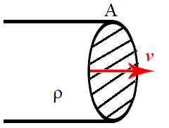
Fig. 13.1 Flux of water passing through a hose pipe, with cross sectional area \(A\)
We can see that the cross sectional area is perpendicular to the velocity in this case, so we define:
where \(\hat{\bf n}\) is a unit vector normal to the surface area \(A\). We can find the rate of mass flowing through the pipe, which is sometimes called the Mass Current \(I_m\) of the water flow, with units of \([\textrm{mass}][\textrm{time}]^{-1}\):
and so we can find the Mass Flux \(\Phi_m\), with units of \([\textrm{mass}][\textrm{length}]^{-2}[\textrm{time}]^{-1}\)
If we increase or decrease the size of the hose, we can figure out the flow rate of the resulting water flow using this mass flux, as we illustrate in Fig. 13.2.

Fig. 13.2 Left panel, flux changes with increase to flow; Middle panel, flux changes with increase to area; Right panel, distorting the area can change the flux through it.
If we increase the size of \(A\), the resulting mass current is smaller (water would flow slower out of hose) and likewise if we decrease \(A\), then the mass current would be larger (water would flower faster out of the hose). We notice that in this hose pipe example, the water flows the cross sectional area \(A\) which is perpendicular to the direction of fluid flow, this may not necessarily be true in other systems.
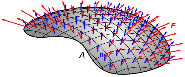
Fig. 13.3 Depiction of some 3D surface area \(A\) decomposed into area elements \(\mathrm{d} A\), with some vector field \(\bf F\) shown in the red. The flux of the vector field is shown in blue as the components of \(\bf F\) in the direction of the normal vectors \(\bf n\) in \(\mathrm{d} A\).
Consider the system shown in Fig. 13.3, where some vector field \(\bf F(x)\) is passing through a surface with area \(A\). We can split up the area into smaller surface elements \(\mathrm{d} A\) and consider the flux \(\Phi\) passing through each of these. In each surface element, we can define a surface normal \(\bf n\) and then just resolve \(\bf F\) into \(\bf F_\parallel\) and \(\bf F_\perp\) components, as shown in Fig. 13.4.
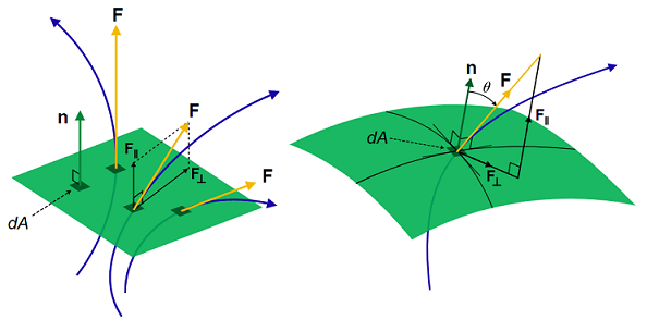
Fig. 13.4 A vector \(\bf F\) passes through some surface (depicted in the green), Left panel, the situation for a flat surface, Right panel the situation for a curved surface. Notice that in each case the setting up a surface normal vector at each position and resolving the vector \(\bf F\) into parallel \(\bf F_\parallel\) and perpendicular \(\bf F_\perp\) components.
Thus we will have the flux for each surface element \(\mathrm{d} A\) as:
and so the total flux will be described by summing up all of these components over the surface, which we can do with a closed surface integral:
13.2. Divergence and Stokes Theorems
For a vector field \(\bf F\) within some volume \(V\), bounded by a surface area \(A\) with surface normal \(\bf n\), as depicted in Fig. 13.5, then we can relate:
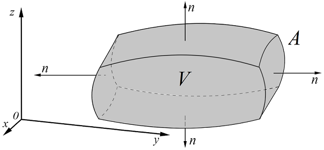
Fig. 13.5 A pictorial look at flux of a vector field \(\bf F\) crossing a bounding area \(A\) which can be related to a divergence \(\nabla \cdot {\bf F}\) within the volume \(V\).
For a vector field \(\bf F\) within boundary \(\ell\) of a surface area \(A\) with surface normal \(\bf n\), as depicted in Fig. 13.6, then we can relate:
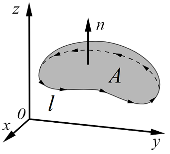
Fig. 13.6 A pictorial look at a vector \({\bf F}\) on the boundary \(\ell\) which can be related to the curl \(\nabla \times {\bf F}\) within the area \(A\).
13.3. Helmholtz Decomposition
The Helmholtz decomposition, shown in Equation (13.1) states that a suitably smooth vector field \(\bf F\) can, in general, be decomposed into two components:
where \(\phi\) is a scalar field, also called the Scalar Potential, and \(\bf A\) is a vector field, also called the Vector Potential.