8. Polarisation of Waves
In our discussion of transverse waves, we outlined that the direction of propogation is perpendicular to the direction of oscillation. In a two dimensional system this means we could align a wave along the \((x,\,y)\) axes, however if we look at three dimensions we see this leaves an ambiguity as any oscillation orientation in the \((y,\,z)\) plane is perpendicular to a wave propogation along the \(x\) axis. The proces of fixing the specific geometric orientation is known as the wave Polarisation.
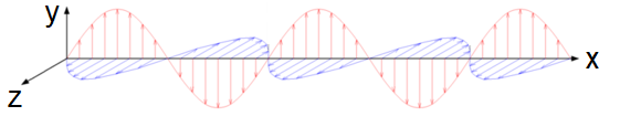
Fig. 8.1 Schematic of two different wave polarisations in the \(y\) (red wave) or \(z\) (blue wave) axes, with wave propogating along the \(x\) axis.
As Fig. 8.1 shows, we can make different choices for the orientation and many materials have the property of being able to filter out or rotate the plane of plane polarised light. But what is the mathematical description of such a phenomena? Lets go back to a travelling wave in three dimensions:
where \({\bf u_0}\) is known as the wave polarisation vector. The orentiation of \({\bf k}\) specifies the direction of progation and \({\bf u_0}\) specifies the direction of oscillation, such that:
If we for instance align a wave to propogate along the \(x\) axis, then we find:
If we pick one of \(u_y,\, u_z\) to be zero also, then the waves are confined to the \(z,\, y\) axes repsectively, giving a Linear polarisation. This condition is not the only solution though, for both \(u_y,\, u_z\) non-zero, these waves can have an alternative polariation state, that of Circular or Elliptical polarisation, as shown in Fig. 8.2.
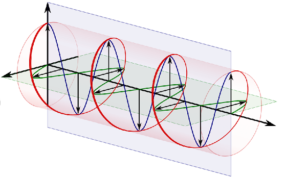
Fig. 8.2 Schematic of two different types of wave polarisations, plane polarisation in green and blue and circular polarisation in red.
If we take the triple vector product of the wave vector and polarisation vector, we find a vector \({\bf S}\) which indicates the flow of energy in the system:
where \(C\) is some constant to be found. To understand how this works, lets pick a choice of linearly polarised placen waves:
then the components of \({\bf S}\) are found by:
which indicates that energy flows along the \(x\) axis - in the same direction as the wave propogration and with a magntiude \(S = |{\bf S}| = C\,k_x\,(u_y)^2 = E_\lambda\) which from Equation (7.3) gives \(C = \pi\,c^2\,\rho_L\).