6.1. Derivation from Waves on a String
Our derivation so far has been done for a longitudinal waves - where the direction of oscillation of the wave is parallel to the direction of propagation
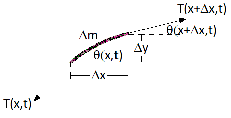
of the wave, as seen in Fig. 4.1. We could however derive the wave equation for an oscaillation travelling on a string, as seen in Fig. 6.1, stretched
out by a tension \(\bf{T}\) and solving the equations of motion. This results in a wave that where the direction of oscillation is perpendicular to the direction of propagation - these
are known as transverse waves.
We will consider a small section of the wire, with \(\Delta x,\,\Delta y,\, \Delta m \rightarrow 0\) and therefore \(\theta \ll 1\).
To begin we resolve forces in the \(y\) direction, which will be unbalanced and therefore have an acceleration term appearing:
(6.1)\[T(x + \Delta x,\,t)\,\sin(\theta(x + \Delta x,\,t)) - T(x,\,t)\,\sin(\theta(x,\,t))
= \Delta m\,\frac{\partial^2 }{\partial t^2} y(x,\,t)\]
The cross section of wire \(\Delta m\) can be reduced down to a mass density (mass per unit length) \(\rho_L\) of the wire (with units kg m\(^{-1}\)) and a length \(\Delta s\):
\[\Delta m = \rho_L \,\Delta s = \rho_L \,\sqrt{\Delta x^2 + \Delta y^2} =
\rho_L \,\Delta x\, \sqrt{1 + \left(\frac{\Delta y}{\Delta x}\right)^2}\]
Looking at Fig. 4.1 we see that:
\[\tan(\theta(x,t)) = \frac{\Delta y}{\Delta x}\]
and therefore we can reduce \(\Delta m\) to:
\[\Delta m = \rho_L \,\Delta x \,\sqrt{1 + \left(\frac{\Delta y}{\Delta x}\right)^2} =
\rho_L \,\Delta x \,\sqrt{1 + \tan^2(\theta(x,t))} = \rho_L \,\Delta x\,\sec(\theta)\]
Rearranging Equation (6.1), we find:
\[\frac{\rho_L}{\cos(\theta)}\,\frac{\partial^2 y}{\partial t^2} =
\frac{T(x + \Delta x,t)\,\sin(\theta(x + \Delta x,\,t)) - T(x,t)\,\sin(\theta(x,\,t))}{\Delta x}\]
and taking the limit of \(\Delta x \rightarrow 0\), we see this is just a partial derivative:
(6.2)\[\frac{\rho_L}{\cos(\theta)}\,\frac{\partial^2 y}{\partial t^2} =
\frac{\partial}{\partial x}\left(T(x,t)\,\sin(\theta(x,t))\right) =
\frac{\partial T}{\partial x}\,\sin(\theta) + T\,\cos(\theta)\,\frac{\partial \theta}{\partial x} \]
If we examine the forces in the \(x\) direction, we see these are balanced:
\[T(x + \Delta x,\,t)\,\cos(\theta(x + \Delta x,\,t)) - T(x,\,t)\,\cos(\theta(x,\,t)) = 0\]
dividing through by \(\Delta x\) and again taking the limit \(\Delta x \rightarrow 0\), we find:
\[\begin{split}\frac{\partial}{\partial x}\left(T(x,t)\,\cos(\theta(x,t)) \right) &= 0 \\
\frac{\partial T}{\partial x}\, \cos(\theta) - T \,\sin(\theta) \,\frac{\partial \theta}{\partial x} &= 0\\
\Rightarrow \frac{\partial T}{\partial x} &= T\,\tan(\theta)\,\frac{\partial \theta}{\partial x}\end{split}\]
Substituting this result into Equation (6.2) and rearranging gives:
\[\begin{split}\rho_L\,\frac{\partial^2 y}{\partial t^2} &=&\, \cos(\theta)\left( T\,\tan(\theta)\,\sin(\theta)\,\frac{\partial \theta}{\partial x} + T\,\cos(\theta)\,\frac{\partial \theta}{\partial x} \right) \\
&=& \,T \,\frac{\partial \theta}{\partial x}\end{split}\]
In the limit of \(\Delta x \rightarrow 0\):
\[\tan(\theta(x,t)) = \frac{\partial y}{\partial x}\]
and taking a \(\partial / \partial x\) derivative:
\[\sec^2(\theta)\frac{\partial \theta}{\partial x} = \frac{\partial^2 y}{\partial x^2}\]
and therefore we find:
\[\frac{\partial^2 y}{\partial t^2} = \frac{T}{\rho_L} \,\cos^2(\theta)\,\frac{\partial^2 y}{\partial x^2}\]
in the limit of \(\theta \ll 1\), with \(c = \sqrt{T/\rho_L}\), this reduces to the wave equation:
\[\frac{\partial^2 y}{\partial t^2} = c^2\,\frac{\partial^2 y}{\partial x^2}\]
We can check the units of \(c\),
\[\begin{split}[\textrm{T}] &=& \, \textrm{N} = \textrm{kg}\,\textrm{m}\,\textrm{s}^{-2}\\
[\rho_L] &=& \,\textrm{kg}\,\textrm{m}^{-1}\\
\Rightarrow \sqrt{[\textrm{T}] / [\rho_L]} &=& \, \sqrt{\textrm{m}^2\,\textrm{s}^{-2}} = \textrm{m}\,\textrm{s}^{-1}\end{split}\]
6.2. Wave Equation in higher dimensions
Given that we now have a wave that can propogate and osciallate in two different dimensions, we can also extend the wave equation to a higher number
of dimensions, packaging the spatial derivatives up into the Laplacian \(\nabla^2\) (sometimes written \(\Delta\)):
(6.3)\[\nabla^2 u = \frac{1}{c^2} \frac{\partial^2 u}{\partial t^2} \]
which in cartesian coordinates takes the form:
\[\begin{split}\nabla &=& \, \left(\frac{\partial}{\partial x},\,\frac{\partial}{\partial y},\, \frac{\partial}{\partial z}\right) \\
\nabla^2 &=& \, \nabla\cdot \nabla = \frac{\partial^2}{\partial x^2} + \frac{\partial^2}{\partial y^2} + \frac{\partial^2}{\partial z^2}\end{split}\]
but in different coordinate systems can take other forms (sometimes we will use the cyclindrical or circular forms instead).
These derivatives are sometimes repackaged up with the d’Alembertian \(\Box\):
\[\Box \,u = \frac{1}{c^2} \frac{\partial^2 u}{\partial t^2} - \nabla^2 u \]
and therefore the wave equation here has the form:
\[\Box \,u = 0\]
We notice that this equation is homogeneous - we could also add a source term on the RHS, although
then it would admit both wave like solutions AND inhomogeous solutions.
6.3. Transverse Wave Energy and Power
Looking at the change total energy \(E\):
\[\Delta E = \Delta K + \Delta U\]
where \(K\) is the total kinetic energy and \(U\) the total potential energy.
\[\begin{split}\Delta K &= \frac{1}{2}\,\Delta m\,v^2 = \frac{1}{2}\,\rho_L\,\Delta x\,
\left(\sqrt{1 + \left(\frac{\partial y}{\partial x}\right)^2}\right)\left(\frac{\partial y}{\partial t}\right)^2 \\
\Delta U &= T(\Delta s - \Delta x) = T\,\Delta x\,\left(\sqrt{1 + \left(\frac{\partial y}{\partial x}\right)^2} - 1\right)\end{split}\]
Recall for transverse waves \(\theta \ll 1\), therefore \(\partial y/\partial x \ll 1\) and so we can do a binomial
expansion:
\[\begin{split}\Delta K &\simeq \frac{1}{2}\,\rho_L\,\Delta x\,\left(\frac{\partial y}{\partial t}\right)^2 + \dots, \\
\Delta U &\simeq T\,\Delta x\,\left(\frac{1}{2}\right)\left(\frac{\partial y}{\partial x}\right)^2 + \dots\\
\Rightarrow \Delta E &= \frac{1}{2} x\,\rho_L\,\left(\left(\frac{\partial y}{\partial t}\right)^2 +
\frac{T}{\rho_L}\left(\frac{\partial y}{\partial x}\right)^2\right)\end{split}\]
and given that \(T / \rho_L = c^2\), we can simplify:
\[\Delta E = \frac{1}{2}\Delta x\,\rho_L\,\left[\left(\frac{\partial y}{\partial t}\right)^2 + c^2
\left(\frac{\partial y}{\partial x}\right)^2\right]\]
If we take the limit \(\Delta x \rightarrow 0\), then we can integrate up to find:
\[\int_0^E \textrm{d}E' = E = \int_0^\lambda \epsilon(x,t) \,\textrm{d}x \]
\[\epsilon(x,\,t) = \frac{1}{2}\,\rho_L\,\left[\left(\frac{\partial y}{\partial t}\right)^2 + c^2
\left(\frac{\partial y}{\partial x}\right)^2\right]\]
and we notice again the energy density term \(\epsilon(x,\,t)\), which matches that for longitundinal waves from Equation (4.5).
If we are deadling with waves propagating in two or three dimensions, with \(y = y({\bf x},\, t)\) then we can switch to using the
gradient operator \(\nabla y\):
\[\epsilon({\bf x},\,t) = \frac{1}{2}\,\rho_L\,\left[\left(\frac{\partial y}{\partial t}\right)^2 + c^2
|\nabla y|^2\right]\]