.md .pdf

repository open issue

Contents

17. Magnetism

17.1. Gauss’s Law for Magnetism

Now that we have got electric fields under control, we should turn our head to magnetic fields. There are clearly some relationships between the two, as well discovering currents, fields and magnets all may interact. Lets consider a bar magnet, as shown in Fig. 17.1, the field lines show the circulation of magnetic field lines from the North pole and into the South pole. A simple way we can observe this is with iron filings or a compass, to trace out the field lines.

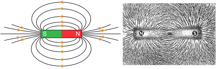
Fig. 17.1 Left Panel, magnetic field lines around a bar magnet, Right Panel, pattern of iron fillings indicating the magnetic field.

We can move from this qualitative understanding of magnetic fields to a mathematical one, using the tools we developed in Chapters 2 and 3. Lets try and understand how Gauss’s law works for magnetic fields:

\[\Phi_B = \iint_A {\bf B} \cdot \mathrm{d} {\bf A}\]

We can see effect of doing this in Fig. 17.2, we see that all the field lines that enter a surface also exit, meaning that the next flux is zero. Additionally if we try to contain all the magnetic field lines within a surface, none of them exit and therefore the flux is zero. Thus we find for magnetic fields:

(17.1)\[\iint_A {\bf B} \cdot \mathrm{d} {\bf A} = 0 \]

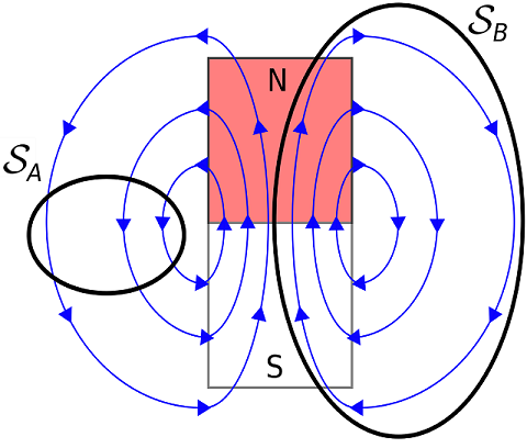
Fig. 17.2 Investigating the magnetic flux through surfaces \(S_A,\, S_B\) around a bar magnet.

We can also interpret this through analogy to Gauss’s law for electric fields:

\[\iint_A {\bf B} \cdot \mathrm{d} {\bf A} \propto \sum_i Q_{magnetic}\]

Where the \(Q_{magnetic}\) would, from the direction of the field lines, represent an isolated north pole \(N\). However around a bar magnet, we see there are only magnetic dipoles, with north and south poles, hence the sum of the all the magnetic “charges” is found to be zero. Gauss’s law for magnetism on its own is not a very useful way to understand magnetic systems. However we can find the magnetic flux through open surfaces to be useful, as we will see later.

17.2. Like and Opposite Poles

We can see that the addition of different magnetic poles can produce magnetic flux, as Fig. 17.3 shows. Drawing a surface between the poles in the middle of the diagram shows that if the net flux is zero, we have the presence of like poles. If however there is a next flux out of (or in to) a surface, then there is a net presence of a north (or south pole) in or near the surface.

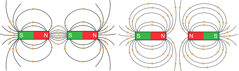
Fig. 17.3 Field lines around bar magnets with like poles (left panel) and opposite poles (right panel) nearby.

Clearly the lowest energy configuration for a system with at least two different orientations of bar magnets is for opposite poles to be neighbouring. These types of systems have been long studied, most notably the Ising Model. We can consider long chains (in 1D) or lattices (in 2D or higher dimensions) of magnets as depicted in Fig. 17.4. The energy figuration of these systems can be studied using the tools of statistical mechanics.

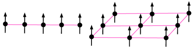
Fig. 17.4 Ising models in 1D (left panel) and 2D (right panel)

17.3. Magnetic Fields, Currents and Biot-Savart Law

Experimentally we observe that a currents flowing in wires produce magnetic fields, as seen in Fig. 17.5. As the iron flings pattern shows, larger currents (here from more current carrying wire) produce stronger magnetic fields, so lets posit \(B \propto I\).

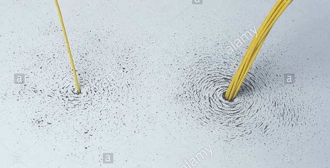
Fig. 17.5 Observed magnetic field from a current carrying wire.

We can see that such as a system displays cylindrical symmetry, as there is rotational invariance around the current, aligned on the \(z\) axis. The magnetic fields direction appears to follow the right handed screw rule, as shown in Fig. 17.6.

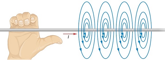
Fig. 17.6 Circular magnetic field from a current carrying wire follows the right hand screw rule

How can we understand the fields created by moving currents in the wire? Lets revisit charges in a line, which we will approximate as a line of charge. We considered the electrostatics of a finite line of charge in Fig. 15.8, which we can modify in Fig. 17.7 with a current \(I\). Lets split up the wire into length elements \(\mathrm{d} {\bf \ell}\), we can imagine contributes to the magnetic field at a given point \(r\) away from the wire.

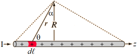
Fig. 17.7 Examining the fields around a finite line of current \(I\), broken up into length elements \(\mathrm{\bf d}\ell = \mathrm{d} \ell\,\hat{\bf z}\) which are aligned along the \(z\) axis.

If we take a conducting wire and pass an electric field \({\bf E}\) through it, free charges will begin to move setting up a current \(I\). These moving charges will follow:

(17.2)\[I = n\,A\,v\,q\]

where \(n\) is the number density of free charges, \(A\) is the conductor cross sectional area, \(v = |{\bf v}|\) is the charge drift velocity and \(q\) is the magnitude of the charge on each charge carrier. If we take the combination of \(I\,\mathrm{d} {\bf \ell}\) then:

(17.3)\[I\,\mathrm{\bf d} \ell = n\,A\,\mathrm{d} \ell\,q\,|{\bf v}|\,\hat{\bf z} = \mathrm{d} N\,q\,{\bf v} = \mathrm{d} Q\,{\bf v}\]

where \(N\) is the number of free charges in the conductor and we have moved the vector dependence from the direction of the length element \(\mathrm{\bf d} \ell\) to the drift velocity \(\bf v\). This suggests we have a current momentum \(Q\,{\bf v}\) in the wire. Lets revisit Equation (15.2) replacing static charges \(\mathrm{d} Q\) with moving charges \(\mathrm{d} Q\,{\bf v}\) and call this the \({\bf B}\) field:

\[\mathrm{d} E = \frac{1}{4\pi\,\epsilon_0}\frac{\mathrm{d} Q \,|{\bf R}|}{|{\bf r}|^3} \longrightarrow \mathrm{d} B = \frac{\mu_0}{4\pi}\,\frac{\mathrm{d} Q\,|{\bf v}|\,|{\bf R}|}{|{\bf r}|^3}\]

Note also that we replaced the electric field constant \(\epsilon_0\) with a magnetic field constant \(\mu_0\). Fig. 17.7 shows \(R = r\sin(\theta)\), hence:

\[\mathrm{d} B = \frac{\mu_0}{4\pi}\,\frac{\mathrm{d} Q\,|{\bf v}|\,|{\bf r}|\,\sin(\theta)}{|{\bf r}|^3}\]

and therefore given the definition of the cross product, we can convert this in to a vector equation:

\[\Rightarrow\mathrm{d} {\bf B} = \frac{\mu_0}{4\pi}\,\frac{\mathrm{d} Q\,{\bf v}\times {\bf r}}{|{\bf r}|^3} = \frac{\mu_0}{4\pi}\,\frac{I\,\mathrm{\bf d}\ell\,\times {\bf r}}{\,|{\bf r}|^3} = \frac{\mu_0}{4\pi}\,\frac{I\,\mathrm{\bf d}\ell\,\times \hat{{\bf r}}}{|{\bf r}|^2}\]

Thus the observed magnetic field from a wire carrying current \(I\) at a distance \({\bf r}\) is given by the Biot-Savart Law:

(17.4)\[{\bf B}({\bf r}) = \frac{\mu_0}{4\pi}\int_C \frac{I \, \mathrm{\bf d}\ell\times\hat{{\bf r}}}{|{\bf r}|^2} \]

which is depicted in Fig. 17.8. We see that the cylindrical symmetry is made explicit, for a wire carrying a current \(I\) in the \(z\) direction, we would measure (at a radial distance \(r\) away from the wire) a magnetic field \({\bf B}\) moving in the \({\bf \theta}\) direction - following the right hand screw rule. We see that each element \(\mathrm{d} \ell\) along the current carrying wire contributes to the total magnetic field \({\bf B}\) at every point \(r\) through the line integral, not just the current element in the \(z\) plane with the magnetic field \(B_\theta\).

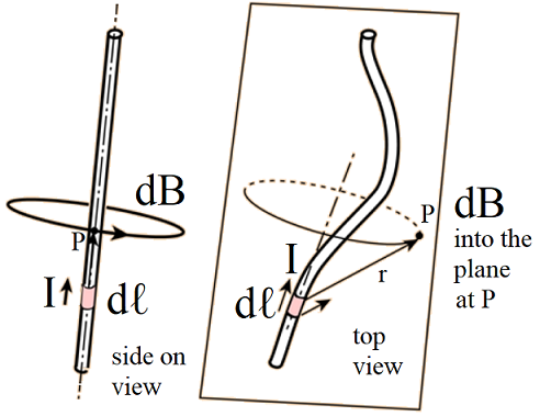
Fig. 17.8 Direction of magnetic field element \(\mathrm{d} {\bf B}\) produced from a wire element \(\mathrm{d} {\bf \ell}\) carrying current \(I\) at a distance \({\bf r}\) from the wire element.

The magnetic field constant \(\mu_0\), also known as the vacuum permeability here is used in the definition of the SI current unit, the Ampère (\(A\)) which is defined to be:

\[\mu_0 = 4\pi\times 10^{-7}\,N\,A^{-2}\]

For an infinite wire, we can use Equation (15.1) and take \(\lambda \rightarrow \lambda\,|{\bf v}| = I\):

(17.5)\[{\bf B} = \frac{\mu_0\,I}{2\pi\,r}\,\hat{{\bf \theta}} \]

17.4. Magnetic Field around a Finite Wire

Solving the Biot-Savart law for different situations looking tricky, however for a finite wire we can think about the system in terms of angles, as depicted in Fig. 17.9.

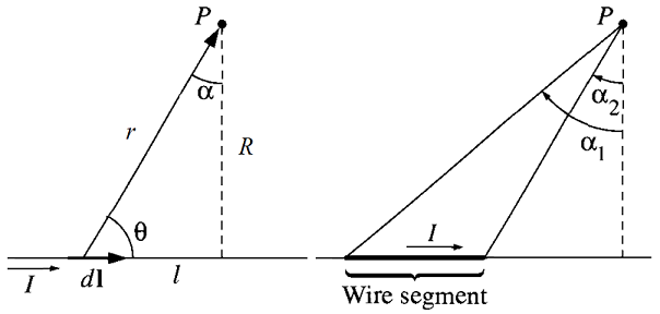
Fig. 17.9 Left Pane - Geometry of a current carrying wire and solving for Biot-Savart law to calculate magnetic field at \(P\), Right Pane - Converting system of wire elements into angles at \(P\).

In this system we can think about the length element of the current, \( \mathrm{\bf d} \ell = \mathrm{d} \ell\,\hat{\bf z}\)

\[\mathrm{\bf d}\ell \times \hat{{\bf r}} = \mathrm{d} \ell \,|\hat{\bf z}|\,|\hat{{\bf r}}|\, \sin(\theta)\,\hat{{\bf \theta}} = \cos(\alpha)\,\mathrm{d} \ell\, \hat{{\bf \theta}}\]

Applying Biot-Savart law here:

\[{\bf B} = \frac{\mu_0}{4\pi}\int_{\mathcal{C}}\frac{I\,\mathrm{\bf d}\ell \,\times \hat{{\bf r}}}{r^2} = \frac{\mu_0\,I}{4\pi}\int_{\mathcal{C}}\frac{\cos(\alpha)}{r^2} \,\mathrm{d} \ell\,\hat{\theta}\]

Given \(\ell = R \tan(\alpha) \Rightarrow \mathrm{d} \ell = R\,\sec^2(\alpha)\,\mathrm{d}\alpha\) and given \(R = r\, \cos(\alpha) \Rightarrow r = R / \cos(\alpha)\):

(17.6)\[\begin{split}{\bf B} &=&\, \frac{\mu_0\,I}{4\pi}\int_{\alpha_1}^{\alpha_2} \frac{\cos(\alpha)\,\cos^2(\alpha)}{R^2}\,R\,\sec^2(\alpha)\, \mathrm{d} \alpha\,\hat{ \theta} \\ &=& \,\frac{\mu_0\,I}{4\pi\,R}\int_{\alpha_1}^{\alpha_2} \cos(\alpha)\,\mathrm{d} \alpha\,\hat{ \theta} \\ &=&\, \frac{\mu_0\,I}{4\pi\,R}\Big[ \sin(\alpha_2) - \sin(\alpha_1)\Big]\,\hat{ \theta}\end{split}\]

Notice that if we take \(\alpha_2 \rightarrow \pi/2,\, \alpha_1 \rightarrow -\pi/2\):

\[{\bf B} = \frac{\mu_0\,I}{2\pi\,R}\,\hat{\theta}\]

then we find the infinite wire result from Equation (17.5).

16. Energy in an Electric Field 18. Magnetic Forces