7. Dispersion Relations and Wave Energy
Now that we have our complex wave solutions to the equation, we can see that plugging in the solutions to the wave equation produce their own equations. Lets start with the simplest wave solution, a 1D right hand moving wave:
Plugging this into the wave equation:
Since we have two roots for \(\omega\) here, we can see that these correspond to either left or right hand moving waves.
Therefore if we usee (7.1) with the proviso that \(\omega = \omega(k) = \pm c\, k\), this describes the travelling wave solutions
in (5.7).
The function \(\omega = \omega(k)\) is known as a dispersion relation. In this case, \(\omega(k)\) is a linear function of \(k\), but in general it could be any function of \(k\). We can also rewrite this linear expression in terms of frequency and wavelegnth \(f = \omega/2\pi, \,\lambda = 2\pi/k\):
which is of course a familiar result!
Looking at the combination of \(\omega/k\), notice it has units of:
and so we see this is a wave speed of some sort!
This is known as the phase velocity of the wave \(v_p\) and describes the rate at which the phase of the wave propagates through space. We can see this by considering
There are other ways to measure the propagation of waves through space, another way that is dimensionally equivalent (but crucially different in the detail) would be
this is known as the group velocity of the wave and describes the velocity with which the overall envelope shape of the wave’s amplitudes (known as the modulation or envelope of the wave) propagates through space.
We can extend this to two and higher dimensions using the gradient operator
Usually these vectors point in the same direction, but there are examples in nature, for instance the anisotropic structure within a crystal, where the two vectors are not parallel.
7.1. Energy and Power of Travelling Waves
Lets again start with a travelling wave \(u\):
the energy density will be given by:
and since \(\omega^2 = c^2\,k^2\) for travelling waves, this simplifies to:
Fig. 7.1 shows the difference in phase between \(u(x,\,t)\) and \(\epsilon(x,\,t)\).
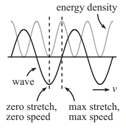
Fig. 7.1 Breakdown of a travelling wave \(u(x,\,t)\) and the associated energy density \(\epsilon(x,\,t)\)
Calculating the energy carried over one wavelength:
where the second step used a double angle trigonometric identity to evaluate the integral:
and we use \(k\lambda = 2\pi\) and by the cyclic nature of \(\sin(x)\), these terms cancel, leaving:
Which suggests \(E_\lambda \propto {u_0}^2\), which is a key result.
Also note that if we did the same analysis with a left travelling wave \(u = u_0\,\exp(i(|k|x + |\omega|\,t))\), the result of Equation (7.2) would be the same, therefore for travelling waves the expression for \(\epsilon\) can be simplifed:
Note this is not true for other types of waves! Likewise the wave power comes out to be:
Notice that this result is related to (7.2) by \(P = c\,\epsilon\) and so the time averaged power is:
where we use \(\omega T = 2\pi\) and by the cyclic nature of \(\cos(x)\), these terms cancel, leaving:
and here we see that \(\langle P \rangle_T\propto {u_0}^2\).
If we think back to oscilaating electrical systems, for an oscillating voltage \(v = V_0\cos(\Omega t)\), the electrical power would be \(P = V^2 / R = {V_0}^2\,\cos^2(\Omega t)/R\) - suggesting the power and oscillation amplitude are related according to \(P \propto {V_0}^2\), which we see is a general fact of travelling wave systems.