10. Matter Waves
10.1. Deriving the Schrödinger Equation
So far we have used the wave equation to construct the dispersion relation for travelling waves, but we can also try to “reverse engineer” this process to construct the wave equation from the form of the dispersion relation.
Lets start with some basic quantum physics, for a particle moving with momentum \(\bf p\), its magnitude \(p = |{\bf p}|\) is related to the de Broglie wavelength \(\lambda\) by:
which we can rewrite in terms of wavevector \(k = |{\bf k}| = 2\pi/\lambda\)
where \(\hbar = h/2\pi\) is the reduced Planck’s constant. Likewise the Planck equation for energy \(E\) and frequency \(f\), can be rewritten using the angular frequency \(\omega = 2 \pi f\):
For a free particle, moving with velocity \({\bf v}\), the only contribution to the energy \(E\) is the kinetic energy \(\frac{1}{2}mv^2\) where \(v^2 = {\bf v}\cdot{\bf v}\) and since \({\bf p} = m{\bf v}\), this means we can rewrite
where \(p^2 = {\bf p}\cdot{\bf p}\). Substituting in the quantum equations (10.1)-(10.2) here gives:
producing a radically different dispersion relation to those we seen up to this point. Indeed this will produce some radically wave behvaiour.
But can we construct a wave equation that similarly produces this? Well if we have the complex form of wave as:
then we can see that in order to get a \(k^2\) here we need a \(\partial^2/\partial x^2\) term in the wave equation and for a \(\omega\) term we need a \(\partial/\partial t\) term in the wave equation.
These will result in an equation of the form:
where \(A = i \hbar\) because \(\partial \psi/\partial t = -i\omega \psi\) and \(B = -\hbar^2/2m\) because \(\partial^2 \psi/\partial x^2 = -k^2 \psi\) producing a one dimensional free particle equation of the form:
If we want to include a potential energy \(V = V(x,t)\) in the system, then we first rewrite the energy as KE + PE:
which results in a modified dispersion relation
and a modified wave equation of the form:
which should look familiar as the Time Dependent Schrödinger Equation (TDSE). If we consider the form of the energy from Equation (10.3), we can interpret the RHS of (10.4) as an energy operator acting of the wave function \(\hat{H}\psi = E\psi\), giving:
which should look familiar as the Time Independent Schrödinger Equation (TISE).
10.2. Relativistic Quantum Mechanics
Unsurprisingly quantum mechanics is not the only relevant physical theory, as bodies get larger and move at relativistic speeds, we need to add in special relativity, given the mass-energy-momentum relation from special relativity,
we can alter the dispersion relation of the wave equation to write a relativistic version of the Schrödinger equation, known as the Klein-Gordon equation. We find this now includes the d’Alembertian operator:
where \(m_0\) is the rest mass of some relativistic particle.
This equation also becomes very useful when studying quantum fields and forms the basis of the Dirac equation.
10.3. Wavepackets
Our simplest form of dispersion relation for travelling waves suggested \(\omega = \pm ck\), which we can write as:
where \(u_n\) is a each waves amplitude. We can generalise this by letting \(u_n = u_n(k)\) and using a continuous spectrum of \(k\) values with a general dispersion relation, therefore:
We call these wave packets, also known sometimes as wave trains or bursts - we can picture them as a larger wave envelope, with smaller localized waves that travel as one unit together, as shown in Fig. 10.1. This infinite set of oscillating waves have different wavelengths, with phases and amplitudes that constructively and destructively interfereonly over different regions of space.
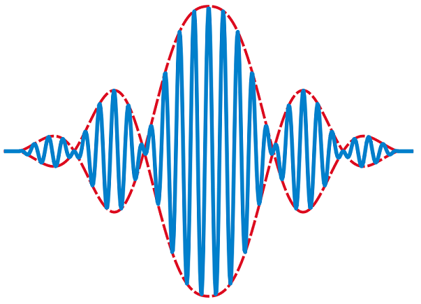
Fig. 10.1 Schematic of a wave packet, with localisation near the centre of the packet.
Each component wave here is a solution of a wave equation and so the entire wave packet is. Depending on the wave equation, the wave packet’s profile may remain constant (no dispersion) or change (dispersion) while propagating.