19. Ampère’s Circuital Law¶

Going back to the magnetic field due to an infinite wire in Equation (17.5):

\[B_\theta = \frac{\mu_0\,I}{2\pi\,r}\]

and recall that this expression (and it’s electric field counterpart in Fig. 15.8) is derived by considering some bounding surface around the line of charge. We found the boundary surface area from the circumference of the cylinders cross sectional area and multiplying by the cylinder length - but in essence we found a bounding contour for moving charges. If we rearrange our expression for the magnetic field:

\[B_\theta\,(2\pi\,r) = \mu_0\,I \Longleftrightarrow B \times (\text{boundary around I}) = \mu_0\,I_\text{{enclosed by boundary}}\]

We can consider breaking up this boundary (containing the current \(I\)) into elements \(\mathrm{d} {\bf \ell}\) and then through a contour integral find the LHS here, this would work therefore for any closed boundary would do, as depicted in Fig. 19.1.

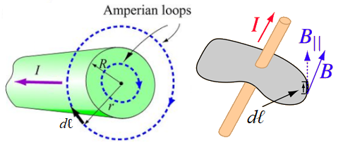
Fig. 19.1 Depiction of Ampère’s circuital law, Left Pane - Applying Ampère’s law on a boundary outside or inside a cylindrical conductor carrying current \(I\).
Right Pane - Current \(I\) enclosed by some boundary in segments \(\mathrm{d} {\bf \ell}\).¶

Thus our expression for Ampère’s Law is given by:

(19.1)¶\[\oint_\ell {\bf B} \cdot\,\mathrm{d} {\bf \ell} = \mu_0 I_{enclosed} \]

19.1. Magnetic Field from a Wire¶

Now lets consider a thick wire, modelled as a cylinder of current \(I\) with cross sectional radius \(R\), as depicted in Fig. 19.1, we see akin to solving Gauss’s law, that there are two regimes of interest:

REGION I: \(r \geq R\)

Applying Ampère’s law, we find the \(I_{enclosed} = I\) here and therefore:

\[\oint {\bf B} \cdot \mathrm{d} {\bf \ell} = B_\theta\,(2\pi\,r) = \mu_0\,I \Rightarrow {\bf B} = \frac{\mu_0\,I}{2\pi\,r}\,\hat{{\bf \theta}}\]

REGION II: \(r < R\)

In order to find the \(I_{enclosed}\) we can see from Equation (17.2) that for a conductor \(I \propto A\) and therefore we can calculate the uniform current density \(\rho = I / A\). Therefore here:

\[\oint {\bf B} \cdot \mathrm{d} {\bf \ell} = B_\theta\,(2\pi\,r) = \mu_0\,I\left(\frac{\,\pi\,r^2}{\pi\,R^2}\right) \Rightarrow {\bf B} = \frac{\mu_0\,I\,r}{2\pi\,R^2}\,\hat{{\bf \theta}}\]

We see that at the boundary of the wire, \(r = R\), these two magnetic field expressions agree. Therefore the magnetic field is given by the piecewise function:

\[\begin{split}{\bf B} = \begin{cases} \mu_0 \,I\, r / 2 \pi\, R^2 \,\hat{\bf \theta} & r < R \\ \mu_0 \,I / 2 \pi\, r \,\hat{\bf \theta} & r \geq R \end{cases}\end{split}\]

and we see a depiction of this in Fig. 19.2. Note that once again the fields expression coincide at the boundary \(r = R\).

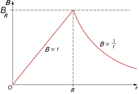
Fig. 19.2 Magnetic field around a thick wire, with cross sectional radius \(R\), note the agreement of the fields at the boundary.¶

19.2. Displacement Current¶

Lets consider a simple circuit with a capacitor, as seen in Fig. 19.3, we could take an Ampère’s law path from the current flowing in to or out of the capacitor to a path cutting through the capacitor.

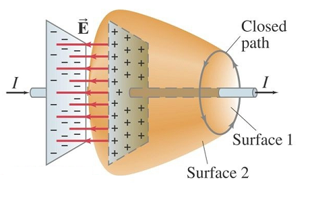
Fig. 19.3 Applying Ampère’s law to a capacitor with no direct current between the plates.¶

This is problematic because there is no current flowing through the capacitor, yet the exact path taken when calculating Ampère’s law should not change the outcome of the expression! What we do see however is an electric field flowing within the capacity, this results in a current flowing at the other end of the capacitor, so we would expect some form of magnetic field contribution. To resolve this, consider the rate of flow of charge \(I = \partial Q/\partial t\) in to or out of the capacitor, from Gauss’s law we know that:

\[Q = \epsilon_0 \iint {\bf E} \cdot \mathrm{d} {\bf A} \Longrightarrow I_{capacitor} = \frac{\partial Q}{\partial t} = \frac{ \partial}{\partial t}\left( \epsilon_0 \iint {\bf E} \cdot \mathrm{d} {\bf A}\right) = \epsilon_0 \iint \frac{ \partial {\bf E}}{\partial t} \cdot \mathrm{d} {\bf A} \]

where we have made use of mixed partial derivatives commuting. Note that we drop the term \(\iint {\bf E}\cdot \mathrm{d} \left(\frac{\partial {\bf A}}{\partial t}\right)\) from the product rule, since the surface \(A\) is constant in time. So our final expression for Ampère’s law may be written:

\[\oint_\ell {\bf B} \cdot\,\mathrm{d} {\bf \ell} = \mu_0 I + \mu_0\epsilon_0 \iint\frac{\partial {\bf E}}{\partial t}\cdot \mathrm{d} {\bf A} \label{eqn:AmperesLawDC}\]

where we have added an additional Displacement Current \(I_D\):

\[I_D = \epsilon_0\iint\frac{\partial {\bf E}}{\partial t}\cdot \mathrm{d} {\bf A}\]

19.3. Magnetic Fields in Coils*¶

In order to make sense of solenoids and other systems with coils of wire, we need to first break down the system of a single circular coil of wire, as shown in Fig. 19.4.

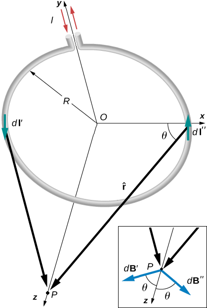
Fig. 19.4 Main Pane - A circular coil of current carrying wire, sitting in the \((x,\,y)\) plane, centered on the origin.
Bottom Pane - At point \(P\) there is a pair-wise cancellation of the magnetic field components in the \((x,\,y )\) plane, leaving only those in the \(z\) direction.¶

In order to find the magnetic field at point \(P\), we can use the Biot-Savart law. Given that the coil sits in the \((x,\, y)\) plane here and we are interested in the magnetic field at a point on the \(z\) axis, the vectors \(\mathrm{d} {\bf \ell}\) and \(\hat{{\bf r}}\) are perpendicular, therefore we have:

\[\mathrm{d} {\bf B} = \frac{\mu_0}{4\pi} \frac{I\,\mathrm{d} \ell}{r^2}\,\hat{{\bf z}} = \frac{\mu_0}{4\pi} \frac{I\,\mathrm{d} \ell}{z^2 + R^2}\,\hat{{\bf z}}\]

A further symmetry we can exploit is there since the direction of the current changes, the direction of \(\mathrm{d} {\bf \ell}'\) is opposite to that of \(\mathrm{d} {\bf \ell}''\). We find that there will a pair-wise cancellation of some of the magnetic field components therefore around the coil, as shown in Fig. 19.4. This means that the components of \({\bf B}\) that are perpendicular to the \(z\) axis will cancel i.e. \({\bf B} \sin(\theta)\) and only the net parallel components, i.e. \({\bf B} \cos(\theta)\) will be non-zero. Therefore the expression we need to find is:

\[{\bf B} = \int_{\mathcal{C}} \frac{\mu_0}{4\pi} \frac{I\,\cos(\theta)\,\mathrm{d} \ell}{z^2 + R^2}\,\hat{{\bf z}} \]

Given that \(\cos(\theta) = R/\sqrt{z^2 + R^2}\), we can simplify:

\[{\bf B} = \frac{\mu_0\,I\,R}{4\pi\,(z^2 + R^2)^{3/2}}\,\int_{\mathcal{C}}\mathrm{d} \ell\,\hat{{\bf z}} \]

Recall that we are integrating around the current loop, not over the \(z\) axis, so we have moved all the constant terms outside the integral, now integrating the segment elements \(\mathrm{d} \ell\) round the loop produces the circumference \(2\pi\,R\):

\[{\bf B} = \frac{\mu_0\,I\,R}{4\pi\,(z^2 + R^2)^{3/2}} \,(2\pi\,R)\,\hat{{\bf z}} = \frac{\mu_0\,I\,R^2}{2(z^2 + R^2)^{3/2}} \,\hat{{\bf z}}\]

At the centre of the loop, \(z = 0\) and therefore:

\[{\bf B} = \frac{\mu_0\,I}{2R} \,\hat{{\bf z}}\]

If we wanted to find the magnetic field at all points in space, the simplification of the cross product in the Biot-Savart law would not be true and the calculation would be fairly complicated! However given we know a fair amount about how magnetic fields behave, we can think about the system qualitatively, as shown in Fig. 19.5.

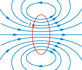
Fig. 19.5 Full magnetic field are a coil of current carrying wire, the straight line through the middle of the coil represents the field calculated along the \(z\) axis.¶

19.4. Magnetic Field in Solenoids*¶

Through superposition of coils, we can find the magnetic field around a solenoid, as shown in Fig. 19.6. The (almost) uniform magnetic field inside a solenoid follows:

\[B = \frac{\mu_0\,N\,I}{L}\]

where \(N\) is the number of turns on the solenoid and \(L\) is the length of the coil. Likewise it is possible to find the magnetic field from a solenoid shaped like a torus, as depicted in Fig. 19.6:

\[B = \frac{\mu_0\,N\,I}{2\pi\,r}\]

where \(r\) is the torus radius.

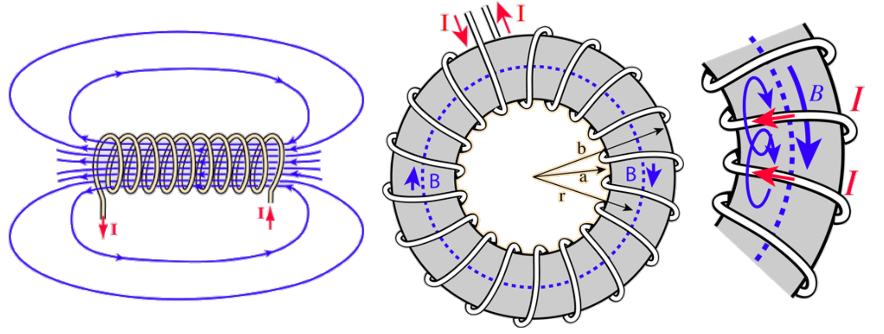
Fig. 19.6 Left Pane - The magnetic field around a current carrying solenoid.
Right Pane - The magnetic field around a current carrying toroidal solenoid.
The magnetic field loops over each turn along the solenoid.¶

19.5. Magnetism in Matter - the \(\bf H\) Field*¶

We might rightly now ask what is the magnetostatic equivalent of the \({\bf D}\) field from electrostatics, describing how magnetic fields permeate through matter. We call this the \({\bf H}\) field and it may be defined as:

\[{\bf H} = \frac{1}{\mu_0}{\bf B} - {\bf M}\]

where \({\bf H}\) is also known as the Magnetic field strength (sometimes Magnetic field intensity), \({\bf B}\) is the magnetic field strength (also sometimes called magnetic flux density) and \({\bf M}\) is the magnetisation vector. We can see the effects of each vector in a bar magnet in Fig. 19.7.

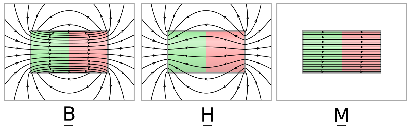
Fig. 19.7 Depiction of different magnetic fields within a bar magnet.¶

In different materials, it is sometimes possible to relate \({\bf M}\) linearly to other fields:

\[{\bf B} = \mu_0\,({\bf H} + {\bf M}) = \mu\,{\bf H} = \mu_0\,(1 + \chi_M)\,{\bf H}\]

where \(\mu\) is the relative permeability and \(\chi_M\) is the magnetic susceptibility.

Electromagnetism, Fluids and Waves