.md .pdf

repository open issue

Contents

15. Solving Electrostatic Systems

15.1. The Tools

• Our first tool for solving electric field system is Gauss’s law:

\[\iint_A {\bf E} \cdot \mathrm{d} {\bf A} = \frac{Q_{enclosed}}{\epsilon_0}\]

In these systems we have to identify the symmetries present in order to use the right co-ordinate system for the bounding surface area \(\bf A\) as well as understand the charge distribution enclosed by this area, \(Q_{enclosed}\).

• Our second tool is superposition of charge, making use of the linearity property of electric fields.

This is usually a good fallback if the system does not have the higher degrees of syummetry that makes using Gauss’s law straightforward. At a point \(\bf r\), in space, the electric field from \(N\) point charges \(Q_i\) at positions \(\bf r_i\) is given by:

\[{\bf E}_{total} = \frac{1}{4 \pi \epsilon_0}\sum_{i=1}^N \frac{Q_i}{|{\bf r-r_i}|^2}\frac{\bf r-r_i}{|\bf r-r_i|}\]

where the final term gives us the unit vector in the relevent direction. If we centre ourselves on the origin, this simplifies to:

\[{\bf E}_{total} = \frac{1}{4 \pi \,\epsilon_0}\sum_{i=1}^N \frac{Q_i}{|{\bf r_i}|^2}\,\hat{\bf r_i}\]

We can also extend this to a continuous distribution of charge:

\[{\bf E}_{total} = \frac{1}{4 \pi \,\epsilon_0}\int_0^Q \frac{\mathrm{d} Q'}{|{\bf r_i}|^2}\,\hat{\bf r_i}\]

and understanding the spatial distribution of \(Q\) can help us to calculate this integral.

15.2. Spheres of Charge

Lets consider the case of a spherical insulator (the key idea here being the charges are fixed), which carries a net charge of \(+Q\). In the first instance we consider that the charge is uniformly distributed throughout the sphere, which has some radius \(a\), as can be seen in Fig. 15.1

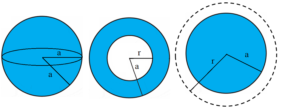
Fig. 15.1 Left: Charged spherical insulator of radius \(a\), Middle: Cross section considering spheres \(r \leq a\),
Right: Cross section considering spheres size \(r \geq a\)

Recall from our discussion of spherical geometries \((r,\,\theta,\, \phi)\), the area normal \(\hat{{\bf n}}\) vector for this Gaussian Sphere will point in the \(\hat{{\bf r}}\) direction, radially outwards, as shown in Fig. 15.2.

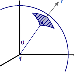
Fig. 15.2 Area normal vector \(\hat{{\bf n}} = \hat{{\bf r}}\) for a sphere.

To find the electric field distribution using Gauss’s law, lets break up the space into three different regimes of interest:

• REGION I: \(r > a\)

Gauss’s law tells us that:

\[\iint {\bf E} \cdot \mathrm{d} {\bf A} = \frac{Q_{enclosed}}{\epsilon_0}\]

Firstly here the charge enclosed by the radius \(r > a\) is the entire charge \(+Q\) carried by the sphere, thus \(Q_{enclosed} = Q\):

\[\iint {\bf E} \cdot \mathrm{d} {\bf A} = \frac{Q}{\epsilon_0}\]

secondly the electric field \({\bf E}\) only has a radial term and no angular dependence:

\[\iint {\bf E} \cdot \mathrm{d} {\bf A} = \iint E_r\mathrm{d} A_r = E_r\iint\mathrm{d} A_r = E_r\,(4 \pi r^2)\]

putting these two facts together we find:

\[E_r\,(4 \pi r^2) = \frac{Q}{\epsilon_0} \Rightarrow E_r = \frac{Q}{4 \pi \epsilon_0 r^2} \]

therefore the full vector expression is:

\[{\bf E} = \frac{Q}{4 \pi \epsilon_0 r^2}\hat{{\bf r} }\]

We notice that this result looks like that of a point charge \(Q\), which for \(r > a\) means we could consider the centre of charge as a point at the centre of the sphere, akin to centre of mass for a large rigid object.

• REGION II: \(r = a\)

Since at \(r=a\) the whole charge is (just) entirely contained, this result matches the condition at \(r > a\), but evaluated at \(r = a\)

\[{\bf E} = \frac{Q}{4 \pi \epsilon_0 a^2}\hat{{\bf r}}\]

This result should match that of the inner and outer electric field - continuity of the field is important so that we are not creating or destroying potential energy.

• REGION III: \(r < a\)

Here we need to find the \(Q_{enclosed}\) at the radius \(r\), this can be found by first finding the uniform charge density within the sphere:

\[\rho = \frac{Q}{\frac{4}{3}\,\pi\, a^3} = \frac{3 Q}{4\,\pi\, a^3} \]

and then multiplying this by the smaller volume of sphere up to radius \(r\):

\[Q_{enclosed} = \frac{3Q}{4\,\pi\, a^3}\left(\frac{4}{3}\,\pi \,r^3\right) = Q \,\left(\frac{r}{a}\right)^3 \]

Putting this into Gauss’s law:

\[\begin{split}\iint {\bf E} \cdot \mathrm{d} {\bf A} &=&\, E_r\,(4 \pi r^2) = \frac{Q}{\epsilon_0} \,\left(\frac{r}{a}\right)^3 \\ \Rightarrow {\bf E} &=&\, \frac{Q}{4 \pi \epsilon_0}\frac{r}{a^3}\hat{{\bf r}}\end{split}\]

Therefore the electric field is given by the piecewise function:

\[\begin{split}{\bf E} = \begin{cases} Q r \,/ \,4 \pi \,\epsilon_0 \,a^3 \,\hat{\bf r} & r < a \\ Q \,/ \,4 \pi \,\epsilon_0\, r^2\, \hat{\bf r} & r \geq a \end{cases}\end{split}\]

and we plot the interior and exterior electric fields in Fig. 15.3. We see that continuity of field is present at the boundary, although very different radial dependencies \(E(r)\) are present inside and outside of the sphere.

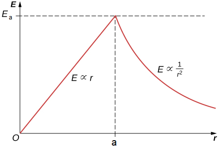
Fig. 15.3 Graph of electric field for uniform insulating sphere interior and exterior.

15.3. Conductors

If we place a conductor in an exterior electric field, the mobile charge carriers now have the possibility to move. This system seeks to reach an equilibrium to minimise their energy configuration. The total electric field inside the conductor is made up of:

\[{\bf E}_{tot} = {\bf E}_{charges} + {\bf E}_{field}\]

and since the charges move until the system reaches a stable equilibrium, the result is

\[{\bf E}_{interior} = - {\bf E}_{field} \quad \Rightarrow \quad {\bf E}_{tot} = (0,\,0,\,0)\]

meaning no more charges will move, which is a stable equilibrium. This is depicted in Fig. 15.4.

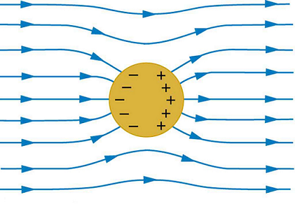
Fig. 15.4 The internal electric field of a conductor that has reached equilbirum after being placed in an exterior electric field.

15.4. Sheets of Charge

We can consider a uniform infinite sheet of charge, carrying a total charge \(Q\) over an area \(A_{tot}\), with a uniform charge for unit area \(\sigma = Q/A_{tot}\). Here we want to find a Gauss’s law surface to find the flux crossing, for a sheet like this we can pick a cylinder, as we see in Fig. 15.5.

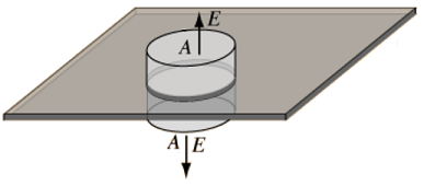
Fig. 15.5 Sheet of charge using a cylinder as our Gaussian surface.

The cylinder has three areas here, two cross sectional area \(A_{r} = \pi\,r^2\) - one for each face and one surface area along the length \(L\) of the cylinder, \(A_{z} = 2 \pi r L\). For the normal to the surface pointing upwards on the top of the sheet (and downwards below the sheet), these point in the \(\text{sign}(z)\hat{{\bf z}}\) direction, depending on which side we are on, so here our Gauss’s law dot product looks like

\[\iint{\bf E} \cdot \mathrm{d} {\bf A} = \iint E_z \,\mathrm{d} A_z = E_z \,A + (-E_z)(-A) = 2 E_z \,A\]

The \(Q_{enclosed}\) here would just be the charge density times the cross section area of the Gaussian cylinder, \(Q_{enclosed} = \sigma \,A\) and therefore:

\[2 E_z \,A = \frac{\sigma\, A}{\epsilon_0} \]

which means we can write a simplified expression here, for \(z > 0 \)

\[ E_z = \frac{\sigma}{2 \epsilon_0} \longrightarrow {\bf E}= \frac{\sigma}{2 \epsilon_0} \hat{\bf z}\]

and equally for \(z < 0\)

\[E_z = \frac{\sigma}{2 \epsilon_0} \longrightarrow {\bf E}= -\frac{\sigma}{2 \epsilon_0} \hat{\bf z}\]

Therefore the electric field is given by the piecewise function:

\[\begin{split}{\bf E} = \begin{cases} -\sigma / 2 \epsilon_0\, \hat{\bf z} & z < 0 \\ \sigma / 2 \epsilon_0 \,\hat{\bf z} & z > 0 \end{cases}\end{split}\]

15.5. Capacitors

A good example for a system where sheets of charge play a role is a capacitor, which we can think of as two sheets of charge, each one carrying an equal and opposite sets of charges \(\pm Q\) as depicted in Fig. 15.6. Obviously this system is idealised, because these sheets of charge are finite - however here we will ignore edge effects.

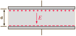
Fig. 15.6 Electric field \(E\) within a capacitor, two plates of area \(A\), top plate at \(z = d\), bottom plate at \(z = 0\), carrying a charge \(\pm Q\).

For two identical plates, each carrying an equal but opposite amount of charge:

\[{\bf E} = {\bf E}_{Q+} + {\bf E}_{Q-}\]

and so there will be a uniform electric field between the plates, in this case in the negative \(z\) direction:

\[{\bf E} = -\frac{\sigma}{2\epsilon_0}\hat{{\bf z}} + \frac{(-\sigma)}{2\epsilon_0}\hat{{\bf z}} = -\frac{\sigma}{\epsilon_0}\hat{\bf z}\]

The electric field outside of the plates is zero, since net charge enclosed will be \(- Q + Q = 0\).

Therefore the electric field is given by the piecewise function:

\[\begin{split}{\bf E} = \begin{cases} 0 & z < 0 \\ -\sigma / \epsilon_0\,\hat{\bf z} & 0 \leq z \leq d \\ 0 & z > d \end{cases}\end{split}\]

Using the defintion of electrostatic potential in Equation (16.2), we can also calculate \(V_E\) between the plates:

\[V_E = -\left(\int_{r_0}^{d}{\bf E} \cdot \mathrm{d} {\bf \ell} -\int_{r_0}^{0}{\bf E} \cdot \mathrm{d} {\bf \ell} \right) = \frac{\sigma\,d}{\epsilon_0} \]

which can be used to find an expression for the capacitance:

\[C = \frac{Q}{V_E} = \frac{\sigma \,A\,\epsilon_0}{\sigma\,d} = \frac{A}{d}\,\epsilon_0\]

Clearly therefore the capacitance can be increased with a larger plates area \(A\) and/or smaller plate separation \(d\). In each case the plates can therefore carry a bigger charge and therefore will result in a larger capacitance \(C\). Likewise if we can increase the size of the permittivity \(\epsilon_0 \rightarrow \epsilon = \epsilon_0(1+\chi_E)\) within a medium, we can increase the capacitence.

15.6. Infinite Lines of Charge

We can consider a uniform infinite line of charges, with charge per unit length \(\lambda\). Again consider a cylinder as our Gauss’s law surface area for flux to cross, but the normal vector now is directed in the radial direction away from the charges and its the long side area that we are concerned with, as depicted in Fig. 15.7.

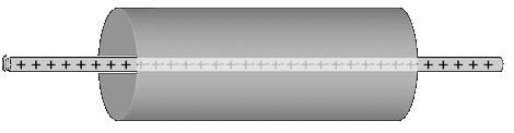
Fig. 15.7 An infinite line of charges, which goes through the origin, with a cylindrical Gaussian surface.

For a cylinder of length \(L\), the area of the long side of the cylinder is \(2 \pi r L\) and the charge enclosed in this area is given by \(\lambda L\), so putting these facts together:

\[\begin{split}\iint {\bf E} \cdot \mathrm{d} {\bf A} &=&\, \iint E_r \,\mathrm{d} A_r = E_r \,(2\pi\, r\, L) = \frac{\lambda L}{\epsilon_0} \\ \Rightarrow E_r &=&\, \frac{\lambda}{2\pi\, \epsilon_0 \,r} \end{split}\]

This gives us an expression for the electric field around an infinite line of charge:

(15.1)\[{\bf E} = \frac{\lambda}{2\pi\, \epsilon_0 \,r} \hat{{\bf r}}\]

Clearly such an object is theoertical, although for very long and thin wires we can approximate the eldctric field for most of the space using this expression.

15.7. Finite Lines of Charge

Equation (15.1) is only true for an infinite line of charge, if we have a finite collection of charges, as depicted in Fig. 15.8, then we loose some of the symmetries of the system, however the superposition method is a better way to proceed here.

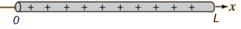
Fig. 15.8 An finite line of charges, with charge density \(\lambda\), with length \(L\), aligned over the \(x\) axis.

15.7.1. Semicircular Arc

Lets start with a simpler problem first though, a semicircular arc of charge, as depicted in Fig. 15.9

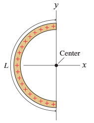
Fig. 15.9 An finite line of charges, with charge density \(\lambda\), arranged in a semicircular arc of length \(L\) and centered on the origin.

What are the symmetries of this semicircular system? Well if we consider a section of the arc, it will carry a charge \(\mathrm{d} Q\) which we can rewrite as \(\mathrm{d} Q = \lambda \mathrm{d} \ell\). Given that for a circular arc \(\ell = r \theta\) and since \(L = \pi r\), therefore

\[\mathrm{d} Q = \frac{\lambda\,L}{\pi} \mathrm{d} \theta\]

where \(\theta\) is an angle that moves round the arc, as we define in Fig. 15.10.

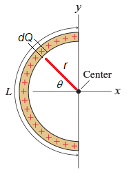
Fig. 15.10 Semicircular arc of charges, centered on the origin, with charge element \(\mathrm{d} Q\), length \(L\), radius \(r\) and angle \(\theta\).

Clearly now we want to integrate over all the charges \(\mathrm{d}Q\) which will involve integrating over all angles \(\mathrm{d} \theta\). Since we are treating these infitesimal charge elements as point charges, the magnitude of the electric field has the form:

\[\mathrm{d} E = \frac{\mathrm{d}Q}{4 \pi\,\epsilon_0\,r^2} = \frac{\pi \,\mathrm{d}Q}{4\,\epsilon_0\,L^2}\]

The direction of the field components however will change depending on whereabouts along the ring we are, clearly are \(\theta = 0\), the field is directed along the \(x\)-axis only:

\[\mathrm{d}{\bf E}_{\theta = 0} = \frac{\pi \,\mathrm{d}Q}{4\,\epsilon_0\,L^2} \,\hat{\bf i} + 0 \,\hat{\bf j}\]

Whilst if we examine the field at \(\theta = -\pi/2\) and \(\theta = \pi/2\), we notice that the electric field will be aligned in the positive and negative \(y\)-axis directions (respectively):

\[\begin{split}\mathrm{d}{\bf E}_{\theta = -\pi/2} &=&\, 0 \,\hat{\bf i} + \frac{\pi \,\mathrm{d}Q}{4\,\epsilon_0\,L^2} \,\hat{\bf j} \\ \mathrm{d}{\bf E}_{\theta =\pi/2} &=&\, 0 \,\hat{\bf i} - \frac{\pi \,\mathrm{d}Q}{4\,\epsilon_0\,L^2} \,\hat{\bf j} \end{split}\]

In fact we see that there will always be a cancellation of the \(y\) components of the electric field from the arc, we can always pair up the components over \(-\pi/2 \leq \theta \leq \pi/2\), this leaves just the \(x\) components:

\[\begin{split}\mathrm{d}{\bf E}_{\theta} &=&\, \frac{\pi \,\mathrm{d}Q}{4\,\epsilon_0\,L^2} \Big[ \cos(\theta) \,\hat{\bf i} + \sin(\theta) \,\hat{\bf j} \Big] \\ \int_0^{\bf E} \mathrm{d}{\bf E}_{\theta} &=&\, \frac{\pi}{4\,\epsilon_0\,L^2} \frac{\lambda\,L}{\pi} \int_{-\pi/2}^{\pi/2} \Big(\cos(\theta)\,\hat{\bf i} + \sin(\theta)\,\hat{\bf j} \Big)\,\mathrm{d} \theta\\ {\bf E} &=&\, \frac{\lambda}{4\,\epsilon_0\,L} \Big[\sin(\theta)\,\hat{\bf i} - \cos(\theta)\,\hat{\bf j}\Big]_{-\pi/2}^{\pi/2} = \frac{\lambda}{2\,\epsilon_0\,L} \,\hat{\bf i} + 0\,\hat{\bf j}\end{split}\]

15.7.2. Rectilinear Rod

Lets return to the rod in Fig. 15.8, we can set this system up in Fig. 15.11, trying to make the rod as symmetric as possible:

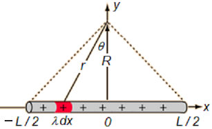
Fig. 15.11 An finite line of charges, with charge density \(\lambda\), with length \(L\), symmetrically aligned over the \(x\) axis. We pick out an element of charge indicated in red, so here \(\mathrm{d} Q = \lambda \,\mathrm{d} x\).

With a line of charge, of length \(L\), aligned along the \(x\) axis, we can look at a point at a distance \(R\) away, aligned halfway along the rod. Once again we can break up this line of charge into infinitesimal chunks, each contributing \(\mathrm{d} Q\) charge and then the overall electric field will be found by superposition. The magnitude of the electric field at a distance \(R\) from the rod appears to be given by:

\[\mathrm{d} E = \frac{\mathrm{d}Q}{4\pi \,\epsilon_0\,r^2}\]

where the length \(r\) can take values between \(R \leq r \leq \sqrt{R^2 + L^2 / 4}\).

In this system, we find that at \(x = 0\), the electric field is only aligned in the \(y\) direction:

\[\mathrm{d} {\bf E}_{x = L/2} = 0\,\hat{\bf i} + \frac{\mathrm{d}Q}{4\pi \,\epsilon_0\,R^2}\,\hat{\bf j}\]

whereas the \(x\) components of the electric field for all the lengths at \(-L/2 \leq x < 0\) and \(0 > x \leq L/2\) will pair up, to cancel out, leaving only the \(y\) components:

\[\begin{split}\mathrm{d} {\bf E} &=&\, \frac{\mathrm{d}Q}{4\pi \,\epsilon_0\,r^2} \Big (\sin(\theta)\,\hat{\bf i} + \cos(\theta)\,\hat{\bf j}\Big)\\ \int_0^{\bf E} \mathrm{d} {\bf E}' &=&\, \frac{\lambda }{4\pi \,\epsilon_0} \int_{-L/2}^{L/2}\Big (\frac{x}{r^3}\,\hat{\bf i} + \frac{R}{r^3}\,\hat{\bf j}\Big)\,\mathrm{d} x\\ {\bf E} &=&\, \frac{\lambda}{4\pi \,\epsilon_0} \int_{-L/2}^{L/2}\Bigg(\frac{x}{(x^2 + R^2)^{3/2}}\,\hat{\bf i} + \frac{R}{(x^2 + R^2)^{3/2}}\,\hat{\bf j}\Bigg)\,\mathrm{d} x \end{split}\]

Where we have used the substitutions \(\sin(\theta) = x/r = x / \sqrt{x^2 + R^2},\, \cos(\theta) = R / r = R / \sqrt{x^2 + R^2}\). We can also use the substitution \(x = R\,\tan(\theta) \Rightarrow \mathrm{d}x = R\,\sec^2(\theta)\) to find:

\[\begin{split}{\bf E} &=&\, \frac{\lambda}{4\pi \,\epsilon_0} \int_{x = -L/2}^{x = L/2}\Big (\frac{R \,\tan(\theta)}{R^3\,\sec^3(\theta)}\,\hat{\bf i} + \frac{R}{R^3\,\sec^3(\theta)}\,\hat{\bf j}\Big) R\,\sec^2(\theta)\,\mathrm{d} \theta \\ &=&\,\frac{\lambda}{4\pi \,\epsilon_0\,R} \int_{x = -L/2}^{x = L/2}\Bigg(\sin(\theta)\,\hat{\bf i} + \cos(\theta)\,\hat{\bf j}\Bigg)\,\mathrm{d} \theta \\ &=&\,\frac{\lambda}{4\pi \,\epsilon_0\,R} \Big[ -\cos(\theta)\,\hat{\bf i} + \sin(\theta)\,\hat{\bf j}\Big]_{x = -L/2}^{x = L/2} \\ &=&\,\frac{\lambda}{4\pi \,\epsilon_0\,R} \Big[ -\frac{R}{(x^2 + R^2)^{1/2}}\,\hat{\bf i} + \frac{x}{(x^2 + R^2)^{1/2}}\,\hat{\bf j}\Big]_{-L/2}^{L/2} \\ &=&\,\frac{\lambda}{4\pi \,\epsilon_0\,R} \Big( 0 \,\hat{\bf i} + \frac{L}{(L^2/4 + R^2)^{1/2}}\,\hat{\bf j}\Big) \end{split}\]

Which results in:

\[{\bf E} = \frac{\lambda\,L }{4\pi \,\epsilon_0\,R\,\sqrt{L^2/4 + R^2}}\,\hat{\bf j}\]

Notice that in the limit of \(L \gg 1\), this would look like:

\[{\bf E} \rightarrow \frac{\lambda}{2\pi \,\epsilon_0\,R}\,\hat{\bf j}\]

which is essentially the result for the infinite line of charge in Equation (15.1).

We note therefore that the relevant expression for the magnitude of the electric field at a distance \(R\) from the rod is found from just the \(y\) component:

(15.2)\[\begin{split}\mathrm{d} E &=&\, \frac{\mathrm{d}Q}{4\pi \,\epsilon_0\,r^2}\,\cos(\theta) = \frac{\mathrm{d}Q\,R}{4\pi \,\epsilon_0\,r^3}\\ \Rightarrow E &=&\, \frac{\lambda}{4\pi \,\epsilon_0}\int_{rod} \frac{R}{r^3}\,\mathrm{d}x = \frac{\lambda}{4\pi \,\epsilon_0\,R} \Bigg[\frac{x}{\sqrt{x^2+R^2}}\Bigg]_{rod}\end{split}\]

15.8. \({\bf D}\) Field*

We find it is possible to have conductors carry a net charge, say \(+Q\), however electrostatic fields do not permeate far through a conductor, the charge is essentially carried at the surface. If we have an oscillating electric field \({\bf E}(\omega)\), then the Skin Effect is observed in a conductor and there is a measurable Skin Depth, \(\delta(\omega)\) of the field in the conductor.

We won’t spend a lot of time discussing electromagnetic fields within transmission media, however one way to investigate how electric fields propagate within a material that isn’t an insulator (or vacuum), say a conductor (or semi-conductor), is to investigate the electric Displacement Field \({\bf D}\). In doing so we must include the effects of frequency dependent permittivity \(\epsilon(\omega)\) in our equations, it is usually more useful to consider the so-called Displacement field \({\bf D}\):

\[{\bf D} = \epsilon(\omega)\,{\bf E} = \epsilon_0\, {\bf E} + {\bf P} = \epsilon_0\,\left(1 + \chi_E \right)\,{\bf E}\]

where \({\bf P}\) is the polarization density and \(\chi_E\) is the electric susceptibility. These expressions let us write Gauss’s law as:

\[\iint {\bf D}\cdot \mathrm{d} {\bf A} = Q_{free}\]

and also mean that the depending the nature of the material and fields in question, the relative permittivity \(\epsilon_r (\omega)\) is related through:

\[\epsilon(\omega) = \epsilon_0\,\epsilon_r(\omega)\]

\(\epsilon(\omega)\) is responsible for effects such as refection and rainbows, producing energy dissipation effects, which we would see in the wave dispersion relation.

14. Electrostatics 16. Energy in an Electric Field