29. The velocity potential¶

In this section:

Is irrotational flow the same thing as potential flow?
Can an irrotational flow be a circulating flow?
When is a potential flow Laplacian?

29.1. Potential flows¶

A potential flow is a velocity field that satisfies any of the following three equivalent conditions. The results are analogous to those for a conservative force field, though the terminology used may be different. For example, we would not talk about the circulation of a force field and would instead say that the field does no work.

Is irrotational (has zero curl)
Has no circulation (is path independent)
Can be written as the gradient of a potential \(\phi\)

Circulation

In fluid dynamics, circulation is the line integral of the velocity field around a closed curve. Any closed curve can be formed of two distinct paths with the same start and end point. If the line integral depends on the path then the flow has non-zero circulation.

Result (1) is immediately obtained from (3) by taking the curl and using the result “curl grad=0” :

(29.1)¶\[\begin{equation}\underline{u}=\nabla\phi \quad \Rightarrow \quad \nabla\times\underline{u}=\nabla\times(\nabla \phi)=\underline{0}\end{equation}\]

Result (2) can be obtained from (1) by appealing to Stokes’ theorem for a surface \(A\) bounded by \(\mathcal{C}\) :

(29.2)¶\[\begin{equation} \oint_{\mathcal{C}}\underline{F}.\mathrm{d}\underline{s} = \iint_A (\nabla \times \underline{F}).\mathrm{d}\underline{A} =0 \end{equation}\]

Warning

It is always true that if a flow has no circulation then it is irrotational. However, the converse is only true if the field is “simply connected”, meaning that it contains no holes. See Example 4 below for a counter-example.

The linking from result (2) to result (3) is called the “Gradient Theorem”. It is not so easy to prove, but is essentially the vector version of the Second Fundamental Theorem of Calculus.

29.2. Calculating the velocity potential¶

To calculate a velocity potential \(\phi\) for an irrotational flow, we need to solve the antiderivative problem

(29.3)¶\[\begin{equation}\underline{u} = \nabla\phi\end{equation}\]

Example 1 : Constant velocity parallel to an axis

\(\underline{u}=(U,0,0)\) is irrotational. It has velocity potential \(\phi=Ux\), since

(29.4)¶\[\begin{equation}\frac{\partial \phi}{\partial x}=U,\quad \frac{\partial \phi}{\partial y}=0, \quad \frac{\partial \phi}{\partial z}=0.\end{equation}\]

Example 2: Stagnation point flow

\(\underline{u}=(\alpha x,-\alpha y,0)\) is irrotational. It has velocity potential \(\phi=\frac{1}{2}\alpha(x^2-y^2)\), since

(29.5)¶\[\begin{equation}\frac{\partial \phi}{\partial x}=\alpha x,\quad \frac{\partial \phi}{\partial y}=-\alpha t, \quad \frac{\partial \phi}{\partial z}=0.\end{equation}\]

29.3. Line integrals for irrotational flows¶

The line integral for an irrotational flow is independent of the path. The result can be obtained from a vector potential:

(29.6)¶\[\begin{equation}\int_{\mathcal{C}}\underline{u}.\mathrm{d}\underline{s}=\int_{\underline{x}_0}^{\underline{x}_1}\nabla\phi.\mathrm{d}\underline{s} = \phi(\underline{x}_1)-\phi(\underline{x}_0) \end{equation}\]

Exercise 29.1

Show that the velocity field \(\underline{u}=(3x^2,3y^2,3z^2)\) is irrotational and that it can be expressed as the gradient of a scalar potential

\[\begin{equation*}\phi=x^3+y^3+z^3 +\mathrm{const.}\end{equation*}\]

Hence, calculate the line integral of this field between \((1,2,1)\) to \((3,2,1)\).

Irrotational: \(\nabla\times\underline{u}=\begin{vmatrix}\underline{e}_x & \underline{e}_y & \underline{e}_z\\\frac{\partial}{\partial x} & \frac{\partial}{\partial y}& \frac{\partial}{\partial z}\\ 3x^2 & 3y^2 & 3z^2\end{vmatrix}=0\underline{e}_x+0\underline{e}_y+0\underline{e}_z\)

\(\underline{u}=\nabla\phi \quad \Rightarrow (3x^2,3y^2,3z^2)=\left(\frac{\partial\phi}{\partial x},\frac{\partial\phi}{\partial y},\frac{\partial\phi}{\partial z}\right)\)

Equating components and integrating gives \(\underline{u}=x^3+y^3+z^3 +\mathrm{const.}\)

Hence, \(\displaystyle \int_{(1,2,1)}^{(3,2,1)}\underline{u}.\mathrm{d}\underline{s} = \phi(3,2,1)-\phi(1,2,1)=26\) (independent of the path)

29.4. Line integrals for flows that are not irrotational¶

For flows that are not irrotational, the line integral generally depends on the path. This isn’t a course on vector calculus, so I won’t make you calculate line integrals but you should take a look at the following examples to see how circulation may arise from a flow that is not irrotational.

Example 3: A flow that is solenoidal but not irrotational

A streamline plot of the velocity field \(\underline{u}=(y^2,x^2,0)\) is shown below. Since the flow is steady, the streamlines are the same as the particle paths.

import numpy as np
import matplotlib.pyplot as plt
x = np.linspace(-2, 2, 10)
y = np.linspace(-2, 2, 10)
X, Y = np.meshgrid(x, y)
U, V = Y**2, X**2

fig,ax=plt.subplots(figsize=(5,5))
ax.axis([-2,2,-2,2])
ax.xaxis.set_ticks([])
ax.yaxis.set_ticks([])
#----------------------------------
start=[ #start points of selected field lines
   [-2,-2],[-2,-1.98],[-2,-1.9],[-2,-1.5],[-2,-0.5],[-2,1.5],
   [-1.98,-2],[-1.9,-2],[-1.5,-2],[-0.5,-2],[1.5,-2]
   ]
#----------------------------------

ax.streamplot(X,Y,U,V,start_points=start,density=10) # stream plot

plt.show()

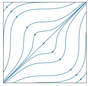
We will calulate the line integral of this field between \((1,0,0)\) to \((0,2,0)\) along two separate path. The result is path-dependent:

\(\displaystyle W=\int_{(1,0,0)}^{(0,2,0)}\underline{u}.\mathrm{d}\underline{s}=\int_{(1,0,0)}^{(0,2,0)}(y^2\mathrm{d}x+x^2\mathrm{d}y)\)

Along the line \(2x+y=2\)
\(\qquad\) Let \(x=t,\) \(y=2-2t\). Then \(\displaystyle W=\int_1^0\left[(2-2t)^2-2t^2\right]\mathrm{d}t=\frac{2}{3}\)
Along a piece of the parabola \(4x+y^2=4\)
\(\qquad\) Let \(y=t,\) \(x=1-\frac{t^2}{4}\). Then \(\displaystyle W=\int_0^2\left[t^2\left(\frac{-t}{2}\right)+\left(1-\frac{t^2}{4}\right)^2\right]\mathrm{d}t= -\frac{14}{15}\)

Example 4: Line vortex flow (a special example)

Line vortex flow \(\underline{u}=\frac{k}{r}\underline{e}_{\theta}\) is irrotational everywhere except at the origin, where it is not defined. If we consider only the region \(r\geq a\) then we have a potential flow:

(29.7)¶\[\begin{equation}\frac{\partial \phi}{\partial r}=0, \quad \frac{1}{r}\frac{\partial \phi}{\partial \theta}=\frac{k}{r}, \quad \frac{\partial \phi}{\partial z} \qquad \Rightarrow \quad \phi=k\theta.\end{equation}\]

We have a field that is irrotational on \(r\geq a\), but it is not conservative. If we calculate the circulation around a closed circuit \(\mathcal{C}\) then we find

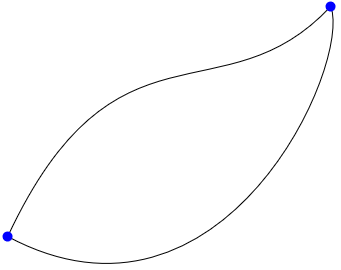
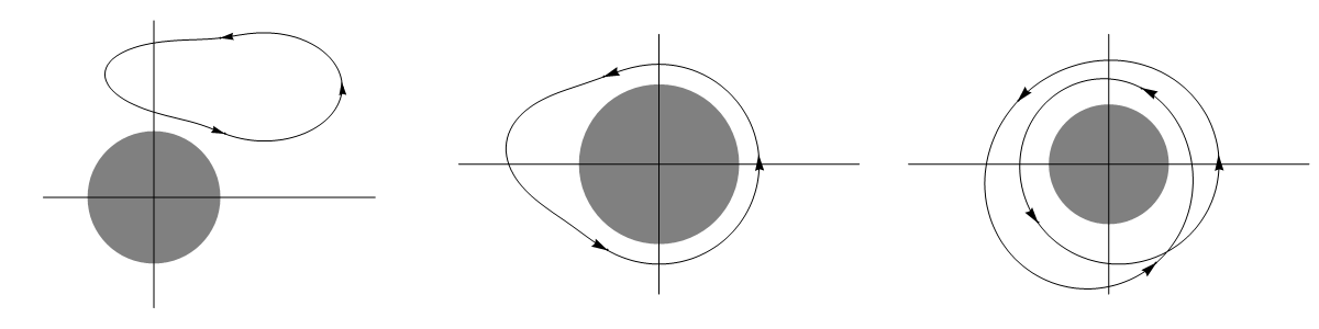
(29.8)¶\[\begin{equation}\Gamma=\int_{\mathcal{C}}(\nabla\phi).d\underline{x}= \int_{\mathcal{C}}\frac{k}{r}r\mathrm{d}\theta = \biggr[k\theta\biggr]_{\mathcal{C}}\end{equation}\]

As we go around any circuit that does not enclose \(r=a\) then \(\theta\) and hence \(\phi\) will return to its original value, so the path integral is zero. However, any closed curve that winds round the origin will have circulation \(\Gamma=2\pi k\). An illustration is provided below. In the first image, the circulation indicated is 0. In the second image, the circulation is \(2\pi k\) and in the third image the circulation is \(4\pi k\).

29.5. Flows that are irrotational and solenoidal¶

Consider an irrotational connected flow, such that the fluid velocity can be expressed as the gradient of a potential:

\[\begin{equation*} \underline{u}=\nabla\phi. \end{equation*}\]

In the case where the flow is also solenoidal, meaning that \(\nabla.\underline{u}=0\), then it is Laplacian:

(29.9)¶\[\begin{equation} \nabla.(\nabla\phi)=0 \quad \Rightarrow \quad \nabla^2\phi=0. \end{equation}\]

Written out in component form, the equation for solenoidal potential flow is

(29.10)¶\[\begin{equation} \frac{\partial^2\phi}{\partial x^2}+\frac{\partial^2\phi}{\partial y^2}+\frac{\partial^2\phi}{\partial z^2}=0. \end{equation}\]

You may recognise this equation as it appears in many other steady state (time-independent) physical contexts including electrostatics, heat conduction and gravitation. It can be quite exciting to recognise that results derived from the heat equation can be applied to the problem of irrotational fluids.

We will see later that the solenoidal assumption is a valid approximation for subsonic flows - where the motion of interest is much less than the speed of sound within the considered fluid. The speed of sound in air on earth is in excess of 1000km/h.

Exercise 29.2

Verify that Laplace’s equation is satisfied by the following potential function:

\[\begin{equation*}\phi=\left[Ce^{kz}+De^{-kz}\right]\sin(kx-\omega t)\end{equation*}\]

This is the velocity potential for travelling waves on a fluid surface.

This is simply an exercise in differentiation:

\(\frac{\partial^2\phi}{\partial x^2}=-k^2\phi, \qquad \frac{\partial^2\phi}{\partial z^2}=k^2\phi\)

Hence, \(\frac{\partial^2\phi}{\partial x^2}+\frac{\partial^2\phi}{\partial z^2}=0\)

Electromagnetism, Fluids and Waves