19. Determinants

The determinant is a single number calculated from a square matrix. The determinant tells us whether the matrix is invertible, as well as a lot of other useful information about the matrix.

We have already seen methods for calculating \(\det(A)\) for \(2\times 2\) and \(3 \times 3\) matrices. In this section we will study properties of the determinant and methods for calculating it for any \(n \times n\) matrix.

19.1. Properties of Determinants

The following three properties can be used to calculate the determinant of any square matrix. We therefore describe them as the ‘defining’ properties of the determinant.

Defining Properties of the Determinant

1. The determinant of the identity matrix is 1.

\[\begin{split}\det(I) = \left|\begin{array}{cccc}1 & 0 & \cdots & 0\\ 0 & 1 & \cdots & 0\\ \vdots & \vdots & \ddots & \vdots\\ 0 & 0 & \cdots & 1\end{array}\right|=1.\end{split}\]

2. The determinant reverses sign when any two rows are exchanged.

\[\begin{split}\left|\begin{array}{ccc} \leftarrow & r_1 & \rightarrow\\ \leftarrow & r_2 & \rightarrow\\ & \vdots & \\ \leftarrow & r_n & \rightarrow\end{array}\right| =-\left|\begin{array}{ccc} \leftarrow & r_2 & \rightarrow\\ \leftarrow & r_1 & \rightarrow\\ & \vdots & \\ \leftarrow & r_n & \rightarrow\end{array}\right|\end{split}\]

3. The determinant is a linear function of each of the rows.

Add two rows \(\implies\) add determinants

\[\begin{split}\left|\begin{array}{ccc} \leftarrow & r_1 + r_1' & \rightarrow\\ \leftarrow & r_2 & \rightarrow\\ & \vdots & \\ \leftarrow & r_n & \rightarrow\end{array}\right| =\left|\begin{array}{ccc} \leftarrow & r_1 & \rightarrow\\ \leftarrow & r_2 & \rightarrow\\ & \vdots & \\ \leftarrow & r_n & \rightarrow\end{array}\right|+ \left|\begin{array}{ccc} \leftarrow & r_1' & \rightarrow\\ \leftarrow & r_2 & \rightarrow\\ & \vdots & \\ \leftarrow & r_n & \rightarrow\end{array}\right|\end{split}\]

Multiply row by \(t\) \(\implies\) determinant is multiplied by \(t\)

\[\begin{split}\left|\begin{array}{ccc} \leftarrow & tr_1 & \rightarrow\\ \leftarrow & r_2 & \rightarrow\\ & \vdots & \\ \leftarrow & r_n & \rightarrow\end{array}\right| =t\left|\begin{array}{ccc} \leftarrow & r_1 & \rightarrow\\ \leftarrow & r_2 & \rightarrow\\ & \vdots & \\ \leftarrow & r_n & \rightarrow\end{array}\right|\end{split}\]

These rules allow us to decompose a determinant into determinants of simpler matrices. For example, using rule 2:

\[\begin{split}\left|\begin{array}{ccc}1&0&0\\0&0&1\\0&1&0\end{array}\right|=-\left|\begin{array}{ccc}1&0&0\\0&1&0\\0&0&1\end{array}\right|=-1.\end{split}\]

Or using rule 3:

\[\begin{split}\left|\begin{array}{ccc}\mathbf{4}&\mathbf{8}&\mathbf{8}\\0&1&1\\0&0&1\end{array}\right|= \mathbf{4}\left|\begin{array}{ccc}\mathbf{1}&\mathbf{2}&\mathbf{2}\\0&1&1\\0&0&1\end{array}\right|\end{split}\]

or

\[\begin{split}\left|\begin{array}{ccc}\mathbf{4}&\mathbf{8}&\mathbf{8}\\0&1&1\\0&0&1\end{array}\right|= \left|\begin{array}{ccc}\mathbf{4}&\mathbf{0}&\mathbf{0}\\ 0&1&1\\0&0&1\end{array}\right|+\left|\begin{array}{ccc}\mathbf{0}&\mathbf{8}&\mathbf{8}\\ 0&1&1\\0&0&1\end{array}\right|.\end{split}\]

We could continue decomposing the matrix by combining row swap, multiplication and addition operations to write it as a sum of multiples of the identity matrix. However this would be very time consuming, so instead we can deduce some further determinant properties from these three. We will not prove all of these properties.

Properties of the Determinant

Let \(A\) be an \(n \times n\) matrix.

4. If one row is equal to another row then \(\det(A)=0\).

5. Adding a multiple of one row to a another row leaves \(\det(A)\) unchanged.

Properties 3 - 5 together mean that the row operations (except multiplying a row by a number) do not affect the determinant. Therefore \(\det(A)=\det(U)\) where \(U\) is the row echelon form (but not the reduced row echelon form) of \(A\).

6. If \(A\) has a zero row then \(\det(A)=0\).

7. If \(A\) is triangular then \(\det(A)\) is the product of the diagonal elements.

8. \(A\) is invertible if and only if \(\det(A)\neq 0\).

9. \(\det(AB) = \det(A)\det(B)\).

10. \(\det(A^{T}) = \det(A).\)

Property 4 follows directly from property 2. Swapping two rows reverses the sign of the determinant, but swapping two equal rows leaves the matrix unchanged. This is only possible if the determinant zero:

\[\det(A) = -\det(A) \implies \det(A) = 0.\]

Exercise 19.1

Prove properties 5, 6 and 7 from properties 1, 2, 3 and 4.

Property 8 follows from the fact that the determinant is the same as its echelon form, and therefore the product of the pivots. But we only have \(n\) nonzero pivots if the matrix is invertible. We will not prove properties 9 - 10 here. For proofs see for example the course text.

Note that every property for the rows can equally be applied to the columns (by transposing, since by property 10 \(|A| = |A^T|\)).

Exercise 19.2

1. Use row operations to calculate the determinant of

\[\begin{split}A = \begin{pmatrix}1&1&1\\1&2&2\\1&2&3\end{pmatrix}.\end{split}\]

2. Let \(B\) be a \((4 \times 4)\) matrix with \(\det(B) = \frac{1}{2}\). Find \(\det(2B)\), \(\det(-B)\), \(\det(B^2)\) and \(\det(B^{-1})\).

19.2. Cofactor Formula for the Determinant of an \(n \times n\) Matrix

The \((n \times n)\) Determinant

Let \(A\) be a \((n \times n)\) matrix with entries \(a_{ij}\) and \(i\) any row of \(A\). Then

\[\det(A) = a_{i1}C_{i1}+\cdots+a_{in}C_{in}\]

where

\[C_{ij} = (-1)^{i+j}\det(M_{ij})\]

and

\(M_{ij}\) is the matrix formed by deleting row \(i\) and column \(j\) from \(A\).

This is a recursive definition of the determinant. In other words, we calculate the determinant of an \((n \times n)\) matrix by calculating the determinant of \((n-1 \times n-1)\) matrices, and so on. The determinant of a \((1 \times 1)\) matrix is defined as the value of its only element. This formula naturally generalises the definition of a \((3 \times 3)\) determinant given in the previous section.

The definition given here calculates determinants by expanding across any row \(i\) of the matrix. If we choose any other row we will get exactly the same value for the determinant. Alternatively, we can expand across columns by choosing any column \(j\):

\[\det(A) = a_{1j}C_{1j}+\cdots+a_{nj}C_{nj}.\]

This method for calculating determinants is very costly for large values of \(n\) so it is unusual to use this formula for general matrices. However, the formula is useful for sparse matrices (matrices with many zeros).

Example

Calculate the determinant of the matrix

\[\begin{split}A=\begin{pmatrix}2&-1&0&0\\-1&2&-1&0\\0&-1&2&-1\\ 0&0&-1&2\end{pmatrix}\end{split}\]

Solution

The matrix has only two nonzero entries in its first row, so only two cofactors \(C_{11}\) and \(C_{12}\) are involved in the determinant:

\[\begin{split}\left|\begin{array}{rrrr}2&-1&&\\-1&2&-1&\\&-1&2&-1\\&&-1&2\end{array}\right|= 2\left|\begin{array}{rrr}2&-1&\\-1&2&-1\\&-1&2\\\end{array}\right|-(-1)\left|\begin{array}{rrr}-1&-1&\\&2&-1\\&-1&2\end{array}\right|.\end{split}\]

Then, expanding each of these \((3\times 3)\) matrices along the first row and first column respectively:

\[\begin{split}\begin{align*}\left|\begin{array}{rrr}2&-1&\\-1&2&-1\\&-1&2\end{array}\right|&= 2\left|\begin{array}{rr}2&-1\\-1&2\end{array}\right|-(-1)\left|\begin{array}{rr}-1&0\\-1&2\end{array}\right|= (2\times3)-2=4,\\ \left|\begin{array}{rrr}-1&-1&\\&2&-1\\&-1&2\end{array}\right|&= -1\left|\begin{array}{rr}2&-1\\-1&2\end{array}\right|= -3. \end{align*}\end{split}\]

Therefore,

\[\det(A)=(2\times 4) - 3 = 5.\]

Exercise 19.3

Calculate \(\det(A)\) where

\[\begin{split}A = \begin{vmatrix}1&0&1&1\\1&0&0&0\\0&1&1&1\\0&1&0&1\end{vmatrix}.\end{split}\]

19.3. Areas and Volumes

The determinant has a useful and intuitive geometrical interpretation as an area or volume. Consider the parallelogram formed by the image of the unit square under a matrix transformation.

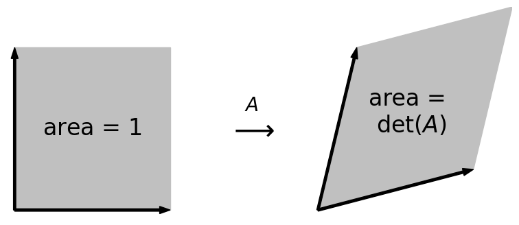
Fig. 19.1 The matrix \(A\) transforms the unit square to a parallelogram with area \(\det(A)\).

It can be shown that the area of this parallelogram is exactly \(\det(A)\). We will not prove this here, but it should be clear that this interpretation of the determinant is consistent with some of its properties. For example:

• The unit square has area 1 \(\Leftrightarrow \det(I)=1\)

• \(A\) transforms both co-ordinate vectors onto a straight line \(\Leftrightarrow\) The area of the parallelogram \(= \det(A)=0\)

There is a similar interpretation in three dimensions and higher.

Geometrical Interpretation of the Determinant

Let \(A\) be an \((n \times n)\) matrix. Then \(\det(A)\) is the (signed) \(n\)-dimensional volume of the \(n\)-dimensional parallelopiped bounded by the transformed co-ordinate vectors.

We can think of the determinant as the factor by which volumes are stretched by the matrix. If the sign is negative then the matrix reverses orientation.

19.4. The Vector and Triple Products

The vector product is a special construction which is only valid in three dimensions. The vector product of two three-dimensional vectors is a vector perpendicular to both of them.

Definition

Let \(u, v \in \mathbb{R}^3\) be two three-dimensional vectors separated by an angle \(\theta\).

The vector product or cross product \( u \times v\) is the vector with magnitude \(\Vert u\Vert \Vert v\Vert |\sin\theta|\) and direction perpendicular to \(u\) and \(v\). It points up or down according to the right hand rule.

The vector product is useful to physicists since it can be used to express physical relationships in three dimensions. For example, if the \(u\) is the position of a mass and \(F\) is a force acting on it, then the turning force or torque is the vector product \(y \times F\). It points along the turning axis perpendicular to both \(u\) and \(F\).

The vector product can be compactly expressed (and easily calculated) using a determinant.

Vector Product as a Determinant

Let

\(u = \begin{pmatrix}u_1\\u_2\\u_3\end{pmatrix}\) and \(v = \begin{pmatrix}v_1\\v_2\\v_3\end{pmatrix}\).

Then

\[\begin{split}u \times v = \left|\begin{array}{ccc}\hat{i}&\hat{j}&\hat{k}\\u_1&u_2&u_3\\v_1&v_2&v_3\end{array}\right|\end{split}\]

where \(\hat{i}, \hat{j}, \hat{k}\) are the three unit coordinate vectors.

Note that here we have used physicists’ notation \(\hat{i}, \hat{j}, \hat{k}\) for the coordinate vectors. Furthermore, we are slightly abusing notation here, because we haven’t explained why it is OK to include vectors inside a matrix. But let us not worry because it works algebraically, and this determinant formula agrees with the definition you have learnt previously. It is also the easiest way to calculate vector products!

Example

Calculate \(u \times v\) where

\(u = \begin{pmatrix}3\\2\\0\end{pmatrix}\) and \(v = \begin{pmatrix}1\\4\\0\end{pmatrix}\).

Solution

Notice that \(u\) and \(v\) are both in the \(xy\) plane, so \(u \times v\) lies on the \(z\)-axis:

\[\begin{split}u \times v = \left|\begin{array}{ccc}\hat{i}&\hat{j}&\hat{k}\\3&2&0\\1&4&0\end{array}\right|= 10\hat{k}=\begin{pmatrix}0\\0\\10\end{pmatrix}\end{split}\]

Since \(u \times v\) is a vector, we can take its dot product with a third vector \(w\), producing the triple product \((u \times v)\cdot w\). It is a ‘scalar’ triple product, because it is a number. In fact it is a determinant.

Definition

Triple product

Let

\(u = \begin{pmatrix}u_1\\u_2\\u_3\end{pmatrix}\), \(v=\begin{pmatrix}v_1\\v_2\\v_3\end{pmatrix}\) and \(w= \begin{pmatrix}w_1\\w_2\\w_3\end{pmatrix}\).

Then

\[\begin{split}(u \times v)\cdot w = \left|\begin{array}{ccc}w_1&w_2&w_3\\u_1&u_2&u_3\\v_1&v_2&v_3\end{array}\right|=\left|\begin{array}{ccc}u_1&u_2&u_3\\v_1&v_2&v_3\\w_1&w_2&w_3\end{array}\right|.\end{split}\]

is the triple product of the three vectors.

Notice that we can put the vector \(w\) on the top or bottom row. The two determinants are equal because it takes two row exchanges to go from one to the other.

The \((u \times v) \cdot w=0 \) exactly when \(u\), \(v\) and \(w\) lie in the same plane:

• \(u\times v\) is perpendicular to the plane when its dot product with \(w\) is zero.

• the determinant is zero when the co-ordinate vectors are squashed onto a plane.

19.5. Solutions to Exercises

Solution to Exercise 19.1

Property 5:

\[\begin{split}\begin{vmatrix}r_1+ar_2\\r_2\\\vdots\\r_n\end{vmatrix}=\begin{vmatrix}r_1\\r_2\\\vdots\\r_n\end{vmatrix}+a\begin{vmatrix}r_2\\r_2\\\vdots\\r_n\end{vmatrix} = \begin{vmatrix}r_1\\r_2\\\vdots\\r_n\end{vmatrix}.\end{split}\]

The first equality uses property 3 (linearity of the determinant) and second uses property 4 (equal rows \(\implies\) zero determinant).

Property 6:

Suppose \(r_1 = \begin{pmatrix}0&\cdots&0\end{pmatrix}\). Then \(r_1 = 0r_1\) so:

\[\begin{split}\begin{vmatrix}r_1\\\vdots\\r_n\end{vmatrix} = \begin{vmatrix}0r_1\\\vdots\\r_n\end{vmatrix} = 0\begin{vmatrix}r_1\\\vdots\\r_n\end{vmatrix} = 0.\end{split}\]

Property 7:

If all diagonal entries are nonzero, then we can remove the off-diagonal zeros using row elimination, which leaves the determinant unchanged (by properties 3-5). This leaves a diagonal matrix. Then use rule 3 to successively each of the diagonal entries:

\[\begin{split}\begin{vmatrix}d_1&&&0\\&d_2&&\\&&\ddots&\\0&&&d_n\end{vmatrix}=d_1\begin{vmatrix}1&&&0\\&d_2&&\\&&\ddots&\\0&&&d_n\end{vmatrix}=d_1\cdots d_n\begin{vmatrix}1&&&0\\&1&&\\&&\ddots&\\0&&&1\end{vmatrix}.\end{split}\]

The result follows from property 1 (\(\det(I)=1\)).

Solution to Exercise 19.2

1.

Use row operations to reduce to echelon form.

\[\begin{split}\begin{vmatrix}1&1&1\\1&2&2\\1&2&3\end{vmatrix}=\begin{vmatrix}1&1&1\\0&1&1\\0&1&2\end{vmatrix}=\begin{vmatrix}1&1&1\\0&1&1\\0&0&1\end{vmatrix} = 1.\end{split}\]

The first equality is because subracting \(r_1\) from \(r_2\) and \(r_3\) does not affect the determinant (property 4). The second equality is because subracting \(r_2\) from \(r_3\) does not affect the determinant (also property 4). The third equality is because the deterimant of a triangular matrix is the product of its diagonal entries (property 7).

2.

\(\det(2B) = 2^4\left(\det(B)\right) = 8\). By property 3, we can factor out \(2\) from each row four times.

\(\det(-B) = (-1)^4\det(B) = \frac{1}{2}\) also by property 3 and factoring out \(-1\) from each row four times.

\(\det(B^2) = \det(BB) = \det(B)\det(B) = \det(B)^2 = \frac{1}{4}\) using property 9.

\(\det(B^{-1}) = 1/\det(B) = 2\) since \(B^{-1}B = I \implies \det(B^{-1})\det(B) = 1\) by property 9 and property 1.

Solution to Exercise 19.3

Expand the \((4\times 4)\) matrix along the second row:

\[\begin{split}\begin{align*} \begin{vmatrix}1&0&1&1\\1&0&0&0\\0&1&1&1\\0&1&0&1\end{vmatrix} &= -1\begin{vmatrix}0&1&1\\1&1&1\\1&0&1\end{vmatrix}\\ &= -1\left(-1\begin{vmatrix}1&1\\0&1\end{vmatrix}+\begin{vmatrix}1&1\\1&1\end{vmatrix}\right)\\ &= -1(-1+0)\\ &= 1 \end{align*}\end{split}\]