5. Line Integrals

If we apply the total differential expression:

\[\nabla f \cdot \mathrm{d}{\bf r} = \mathrm{d}f\]

and now try to integrate this:

\[\int \,\mathrm{d}f = \int\,\nabla f \cdot \mathrm{d}{\bf r}\]

we see that this can be thought of doing the scalar product between two vectors \({\bf F}\) and \(\mathrm{d}{\bf r}\) before finally integrating:

\[\int {\bf F}\cdot \mathrm{d}{\bf r}\]

We call integrals of this kind line integrals or otherwise called contour integrals.

Definition

We can define:

\[\int_{\mathcal{C}} {\bf F(r)} \cdot \mathrm{d}{\bf r}\]

which we call a vector line integral. This is an integral through coordinate space along a contour, here denoted \(\mathcal{C}\).

For some vector field:

\[{\bf F(r)} = \hat{\bf x}\,P({\bf r}) +\hat{\bf y}\,Q({\bf r}) +\hat{\bf z}\,R({\bf r})\]

this simplifies to:

\[\int_{\mathcal{C}} {\bf F(r)} \cdot \mathrm{d}{\bf r} = \int_{\,\mathcal{C}} \left(F\,\mathrm{d}x + G\,\mathrm{d}y + R\,\mathrm{d}z \right)\]

We notice that that this is a scalar, found from scalar product of \(\bf F\) with the differential line element \(\mathrm{d}{\bf r}\) along the path \(\mathcal{C}\).

We can also think about a scalar line integral:

\[\int_{\mathcal{C}} f(r)\, \mathrm{d}s\]

where \(\mathrm{d}s\) is the infinitesimal arc length element, which is given by:

\[\begin{split}\mathrm{d} {\bf r} &= \hat{\bf x}\,\mathrm{d}x +\hat{\bf y}\,\mathrm{d}y +\hat{\bf z}\,\mathrm{d}z\\ \mathrm{d} s &= |\mathrm{d} {\bf r}|= \sqrt{\mathrm{d}x^2 + \mathrm{d}y^2 + \mathrm{d}z^2}\end{split}\]

If we pick a closed path through the vector field, we call this a loop integral:

\[\oint_{\mathcal{C}} {\bf F(r)} \cdot \mathrm{d}{\bf r}\]

What does a line integral actually do? We can think about moving along some line which we denoted \(\mathcal{C}\), broken up into infintesimal sections \(\mathrm{d} r\), as depicted in Fig. 5.1.

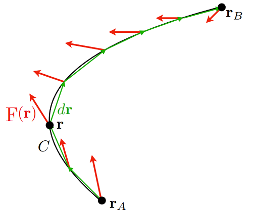
Fig. 5.1 Ilustration of a line integral, with \(\int_{\mathcal{C}} {\bf F}({\bf r})\cdot \mathrm{d}{\bf r}\)

5.1. Parameterising and evaluating integrals

Whilst our expressions for line integrals are powerful, they also do not really explain how we can go about calculating integrals.
To see how we can go about this, we need to think about how to parameterise our paths (contours) through coordinate space. Once we have a good way to think about parameterising our contours, we will aim to use a change of variable to evaluate the integrals.

5.1.1. Parameterising contours

Lets think about different contours between the points \(A(-1,\,1)\) and \(B(1,\,1)\), as depicted in Fig. 5.2.

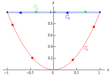
Fig. 5.2 Ilustration of a three contours \(C_1,\, C_2,\, C_3\) between the points \(A(-1,\,1)\) and \(B(1,\,1)\).

If we travel along contour \(C_1\) which follows \(y = x^2\) for \(-1\leq x \leq 1\), whilst we can also travel along contour \(C_2\) which takes \(y = 1\) for \(-\ leq x \leq 1\) and \(C_3\) which is a contour with theopposite direction. These sorts of contours are problematic to describe using just \(x,\,y\) variables and the orientation of the contours is also not well captured.

We can use some standard parameterisation schemes to capture all the relevant details here:

• For straight lines over points \((x_0,\, y_0,\, z_0)\) to \((x_1,\, y_1,\, z_1)\), we can parameterise this contour using:

\[\begin{split}x &= x_1 (1-t) + x_1 t\\ y &= y_1 (1-t) + y_1 t\\ z &= z_1 (1-t) + z_1 t\end{split}\]

where \(0 \leq t \leq 1\).

Worked example

For the contour \(C_2\) between \(A(-1,\,1)\) and \(B(1,\,1)\), we can see that with \(0 \leq t \leq 1\):

\[\begin{split}x &= 2t-1 \\ y &= 1\end{split}\]

and for the contour \(C_3\) between \(B(1,\,1)\) and \(A(-1,\,1)\), we can see that with \(0 \leq t \leq 1\):

\[\begin{split}x &= 1-2t \\ y &= 1\end{split}\]

• For functions \(y = f(x)\) over range \(a \leq x \leq b\), i.e. over \((a,\, f(a)) \rightarrow b,\, f(b)\), we can parameterise using \(a \leq t \leq b\):

\[\begin{split}y &= f(t) \\ x &= t\end{split}\]

We note that here we can also go in the opposite orientation \((b,\, f(b)) \rightarrow (a,\, f(a))\) by switching \(x = t \rightarrow x = -t\).

Worked example

For the contour \(C_1\) between \(A(-1,\,1)\) and \(B(1,\,1)\), we can see that with \(-1 \leq t \leq 1\):

\[\begin{split}y &= t^2 \\ x &=t\end{split}\]

and in order to reverse the contour direction we can just switch \(x = t \rightarrow x = -t\).

• For a circular path (or circular arc) between points \((a,\, b)\) and \((c,\, d)\) such that \(a^2 + b^2 = c^2 + d^2 = r^2\), we can parameterise using \( t_i \leq t \leq t_f\):

\[\begin{split}x &= r\,\cos(t) \\ y &= r\,\sin(t)\end{split}\]

For scalar line integrals, the direction we travel along the contour does not change the result:

\[\int_{-\mathcal{C}}f\,\mathrm{d}s = \int_{\mathcal{C}} f\,\mathrm{d}s\]

this is because the length element \(\mathrm{d}s = |\mathrm{d}{\bf r}|\) is taken from the magnitude of a vector, so any changes in the orientation are washed out in this.

For vector line integrals, the direction we travel along the contour does change the result:

\[\int_{-\mathcal{C}} {\bf F}\cdot \,\mathrm{d}{\bf r} = -\int_{\mathcal{C}} {\bf F}\cdot \,\mathrm{d}{\bf r} \]

and given that for \(Q = R = 0\), we can do a line integral in \(x\), or similarly for \(y\) \(z\):

\[\begin{split}\int_{-\mathcal{C}} P({\bf r})\,\mathrm{d}x &= -\int_{\mathcal{C}} P({\bf r})\,\mathrm{d}x\\ \int_{-\mathcal{C}} Q({\bf r})\,\mathrm{d}y &= -\int_{\mathcal{C}} Q({\bf r})\,\mathrm{d}y\\ \int_{-\mathcal{C}} R({\bf r})\,\mathrm{d}z &= -\int_{\mathcal{C}} R({\bf r})\,\mathrm{d}z\end{split}\]

5.1.2. Evaluating line integrals

If we can find one variable \(t\) which will effectively parameterise the path through the (scalar or vector) field, then our expression simplify:

\[\begin{split}\int_{\mathcal{C}} f({\bf r})\,\mathrm{d}s = \int_{t=a}^{t=b} \left(f({\bf r}(t))\,\frac{\mathrm{d}s}{\mathrm{d}t}\right)\,\mathrm{d}t \\ \int_{\mathcal{C}} {\bf F}({\bf r})\cdot \mathrm{d}{\bf r} = \int_{t=a}^{t=b} \left({\bf F}({\bf r}(t))\cdot\frac{\mathrm{d}{\bf r}}{\mathrm{d}t} \right)\,\mathrm{d}t\end{split}\]

where the infinitesimal coordinate vector derivatives are given by:

\[\begin{split}\frac{\mathrm{d}{\bf r}}{\mathrm{d}t} &= \hat{\bf x}\,\frac{\mathrm{d}x}{\mathrm{d}t} + \hat{\bf y}\,\frac{\mathrm{d}y}{\mathrm{d}t} + \hat{\bf z}\,\frac{\mathrm{d}z}{\mathrm{d}t}\\ \frac{\mathrm{d}s}{\mathrm{d}t} &= \left|\frac{\mathrm{d}{\bf r}}{\mathrm{d}t} \right| = \sqrt{\left(\frac{\mathrm{d}x}{\mathrm{d}t}\right)^2 + \left(\frac{\mathrm{d}y}{\mathrm{d}t}\right)^2 + \left(\frac{\mathrm{d}z}{\mathrm{d}t}\right)^2}\end{split}\]

Worked examples

1. Evaluate the scalar line integral \(\int_{\mathcal{C}} (x^2 + y^2)\,\mathrm{d}s\) over the contours:

a. A straight line linking \((1,\,0) \rightarrow (-1,\,0)\).

Here we can use the straight line parametrisation for \(0 \leq t \leq 1\):

\[\begin{split}x &= x_0(1-t) + x_1 t = 1-t - t = 1-2t \\ y &= y_0(1-t) + y_1 t = 0\end{split}\]

Then we can rewrite the integrand in this parameterisation:

\[\begin{split}x^2 + y^2 &= (1-2t)^2 + 0^2 = 1 - 4t + 4t^2 \\ \frac{\mathrm{d}x}{\mathrm{d}t} &= -2\\ \frac{\mathrm{d}y}{\mathrm{d}t} &= 0\\ \frac{\mathrm{d}s}{\mathrm{d}t} = \sqrt{(-2)^2 + 0^2} = 2\end{split}\]

Finally lets evaluate the integral:

\[\int_0^1 2(1 - 4t + 4t^2)\,\mathrm{d}t = \left[2t - 4t^2 + \frac{8}{3}t^3\right]_0^1 = \frac{2}{3}\]

b. A semi-circular arc linking \((1,\,0) \rightarrow (-1,\,0)\) in the top half of the plane.

Here we can use polar coordinates, with \(r=1\)

\[\begin{split}x &= \cos(\theta) \\ y &= \sin(\theta)\end{split}\]

with \(0 \leq \theta \leq \pi\).

Rewriting the integrand in this parameterisation:

\[\begin{split}x^2 + y^2 &= (\cos(\theta))^2 + (\sin(\theta))^2 = 1 \\ \frac{\mathrm{d}x}{\mathrm{d}t} &= -\sin(\theta)\\ \frac{\mathrm{d}y}{\mathrm{d}t} &= \cos(\theta)\\ \frac{\mathrm{d}s}{\mathrm{d}t} &= \sqrt{(-\sin(\theta))^2 + (\cos(\theta))^2} = 1\end{split}\]

Finally lets evaluate the integral:

\[\int_0^\pi (1)\,(1)\mathrm{d}\theta = \Big[\theta\Big]_0^\pi = \pi\]

We can picture this system by plotting the surface \(z = x^2 + y^2\):

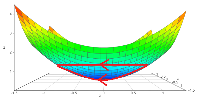
Fig. 5.3 Ilustration of a parabolic surface \(z = x^2 + y^2\) with the contours in (a) and (b) shown.

We can see that the distance for contour (a) is shorter than for contour (b) and since the scalar function is \(x^2\) along both contours, the integral is the weighted sum of \(x^2\) along each of these lengths, hence it makes sense that \(I_a < I_b\).

2. Evaluate the vector line integral \(\int_{\mathcal{C}} {\bf F}\cdot \mathrm{d}{\bf r}\) for \({\bf F} = xz\,\hat{\bf x} - yz\,\hat{\bf z}\) along the line linking \((-1,\,2,\,0) \rightarrow (3,\,0,\,1)\).

Here we need a parameterise the line over \(0 \leq t \leq 1\):

\[\begin{split}x &= x_0(1-t) + x_1 t = -1(1-t) + 3(t) = 4t - 1\\ y &= y_0(1-t) + y_1 t = 2(1-t) + 0(t) = 2-2t\\ z &= z_0(1-t) + z_1 t = 0(1-t) + 1(t) = t\end{split}\]

Using this we can rewrite the variables in terms of \(t\):

\[\begin{split}{\bf F} &= t(4t-1)\,\hat{\bf x} - t(2-2t)\,\hat{\bf z}\\ \frac{\mathrm{d}{\bf r}}{\mathrm{d}t} &= 4\,\hat{\bf x} -2\,\hat{\bf y} + \hat{\bf z}\end{split}\]

and so we can find the dot product:

\[{\bf F}\cdot \frac{\mathrm{d}{\bf r}}{\mathrm{d}t} = 4(4t^2-t) - 2t(1-t) = 18t^2 - 6t\]

which we can then just integrate:

\[\int_0^1 (18t^2 - 6t)\,\mathrm{d}t = \Big[6t^3 - 3t^2\Big]_0^1 = 3\]

Further worked examples

1. Find the line integral of the vector field:

\[\begin{split}{\bf G(r)} = \begin{pmatrix} xy\\ -y^2 \end{pmatrix}\end{split}\]

over the following contours:

a. Straight line path \((0,\,0) \rightarrow (1,\, 2)\)

The path followed can be parameterised over \(0\ leq t \leq 1\) by:

\[\begin{split}x &= x_0(1-t) + x_1t = 0(1-t) + 1t = t\\ y &= y_0(1-t) + y_1t = 0(1-t) + 2t = 2t\end{split}\]

Thus \({\bf G}({\bf r}(t))\) will be:

\[\begin{split}{\bf G}({\bf r}(t)) = \begin{pmatrix} 2t^2 \\ -4t^2 \end{pmatrix}\end{split}\]

and \({\bf r'}(t)\) is given by:

\[\begin{split}{\bf r}'(t) = \begin{pmatrix} 1 \\ 2 \end{pmatrix}\end{split}\]

so the line integral is found by:

\[\begin{split}I &= \int_{\mathcal{C}} {\bf G}(r) \cdot \mathrm{d}{\bf r} = \int_0^1 {\bf G}({\bf r}(t)) \cdot {\bf r}'(t)\,\mathrm{d}t = \int_0^1 \begin{pmatrix} 2t^2 \\ -4t^2 \end{pmatrix} \cdot \begin{pmatrix} 1 \\ 2 \end{pmatrix} \mathrm{d}t \\ &= \int_0^1 \left( 2t^2 - 8t^2 \right)\,\textrm{d}t = -\int_0^1 6t^2 \,\textrm{d}t = \Big[ -\frac{6}{3}t^3\Big ]_0^1 = -2\end{split}\]

b. Curved path following \(y = x^2\) for \(0 \leq x \leq 1\)

So the parameterisation for \(0 \leq t \leq 1\) is:

\[\begin{split}{\bf r}(t) = \begin{pmatrix} t \\ t^2 \end{pmatrix}\end{split}\]

Thus \({\bf G}({\bf r}(t))\) will be:

\[\begin{split}{\bf G}({\bf r}(t)) = \begin{pmatrix} t^3 \\ -t^4 \end{pmatrix}\end{split}\]

and \({\bf r'}(t)\) is given by:

\[\begin{split}{\bf r}'(x) = \begin{pmatrix} 1 \\ 2t \end{pmatrix}\end{split}\]

so the line integral is found by:

\[\begin{split}I &= \int_{\mathcal{C}} {\bf G}(r) \cdot \mathrm{d}{\bf r} = \int_0^1 {\bf G}({\bf r}(t)) \cdot {\bf r}'(t)\,\mathrm{d}t = \int_0^1 \begin{pmatrix} t^3 \\ -t^4 \end{pmatrix} \cdot \begin{pmatrix} 1 \\ 2t \end{pmatrix} \mathrm{d}t \\ &= \int_0^1 \left( t^3 - 2t^5 \right)\,\textrm{d}t = \Big[\frac{1}{4}t^4 - \frac{1}{3}t^6 \Big ]_0^1 = -\frac{1}{12}\end{split}\]

c. Curved path following \(y = x^{1/2}\) over \(0 \leq x \leq 1\)

So the parameterisation for \(0 \leq t \leq 1\) is:

\[\begin{split}{\bf r}(t) = \begin{pmatrix} t \\ t^{1/2} \end{pmatrix}\end{split}\]

Thus \({\bf G}({\bf r}(t))\) will be:

\[\begin{split}{\bf G}({\bf r}(t)) = \begin{pmatrix} t^{3/2} \\ -t \end{pmatrix}\end{split}\]

and \({\bf r'}(x)\) is given by:

\[\begin{split}{\bf r}'(t) = \begin{pmatrix} 1 \\ \frac{1}{2} t^{-1/2} \end{pmatrix}\end{split}\]

so the line integral is found by:

\[\begin{split}I &= \int_{\mathcal{C}} {\bf G}(r) \cdot \mathrm{d}{\bf r} = \int_0^1 {\bf G}({\bf r}(t)) \cdot {\bf r}'(t)\,\mathrm{d}t = \int_0^1 \begin{pmatrix} t^{3/2} \\ -t \end{pmatrix} \cdot \begin{pmatrix} 1 \\ \frac{1}{2} t^{-1/2} \end{pmatrix} \mathrm{d}t \\ &= \int_0^1 \left( t^{3/2} - \frac{1}{2}t^{1/2} \right)\,\textrm{d}t = \Big[\frac{2}{5}t^{5/2} - \frac{1}{3}t^{3/2} \Big ]_0^1 = \frac{1}{15}\end{split}\]

5.2. Conservative vector fields

In the case of a conservative vector field \({\bf F} = \nabla f\), then we find that the line integral is actually path independent, something which allows us to dramatically simplify calculating it in some cases. To see this fact, go back to the total derivative:

\[\nabla f \cdot \mathrm{d}{\bf r} = \mathrm{d}f\]

If this is true, then when we calculate the line integral of a conservative vector field:

\[\int_{\mathcal{C}} \nabla f \cdot \mathrm{d}{\bf r} = \int_{f_{initial}}^{f_{final}} \mathrm{d}f = \Big[ f\Big]_{f_{initial}}^{f_{final}} = f_{final} - f_{initial}\]

over some points \(f_{initial} \rightarrow f_{final}\) which correspond to the points \(a \leq t \leq b\) in the parameterised version of the line integral.

Hence this answer only depends on the starting/ending values of the path integral, not the path taken.