18. Inverses

18.1. Inverse Functions

The inverse of a function \(f\) is a function which ‘undoes’ the action of \(f\). In other words if \(g\) is an inverse of \(f\) then \(g(f(x)) = x\) for all values of \(x\) in the domain of \(f\) and \(f(g(y)) = y\) for all values of \(y\) in the domain of \(g\).

If \(g\) is the inverse of \(f\) then we write \(g = f^{-1}\).

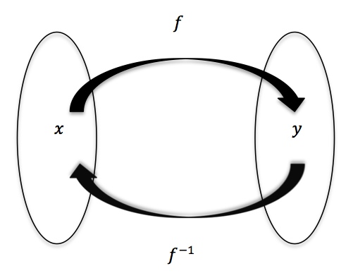
Fig. 18.1 The inverse of a function \(f\) is the function \(f^{-1}\) for which \(f^{-1}(f(x)) = x\) and \(f(f^{-1}(y)) = y\).

Exercise 18.1

For each of the functions below, state whether it has an inverse and if so write it down.

1. \(f:\mathbb{R} \rightarrow \mathbb{R}\), \(f(x) = x^2\).

2. \(g:\mathbb{R}^+ \rightarrow \mathbb{R}^+\), \(g(x) = x^2\), where \(\mathbb{R}^+\) is the set of positive real numbers.

3. \(h:\mathbb{R}^2 \rightarrow \mathbb{R}\), \(h(x, y) = x + y\).

18.2. Matrix Inverses

Since a matrix represents a linear transformation, which is a function, we can consider if a matrix has an inverse. For example, consider the \((2 \times 2)\) matrix \(R_{\pi/2}\) which represents a \(\pi/2\) anticlockwise rotation about the origin:

\[\begin{split}R_{\pi/2} = \begin{pmatrix}0 & -1 \\1 & 0\end{pmatrix}.\end{split}\]

Its inverse is a \(\pi/2\) clockwise rotation about the origin, represented by the following matrix:

\[\begin{split}R_{3\pi/2} = \begin{pmatrix}0 & 1 \\-1 & 0\end{pmatrix}.\end{split}\]

In general, if \(A\) is an \(n \times n\) matrix and \(B\) is its inverse, then \(B\) is also an \((n \times n)\) matrix which satisfies

\[ABx = x\]

for all \(x \in \mathbb{R}^n\).

In other words, \(AB\) is a matrix which leaves \(x\) unchanged. The only matrix which leaves \(x\) unchanged is the identity matrix \(I\), and so we have the following definition of the inverse matrix.

Definition

Let \(A\) be an \((n \times n)\) square matrix. If there is an \((n \times n)\) matrix \(B\) such that

\[AB = BA = I_n\]

then \(A\) is invertible and \(B\) is the inverse of A.

We write \(B = A^{-1}\).

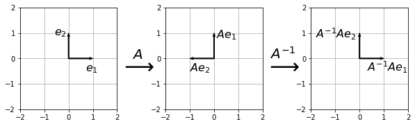
Fig. 18.2 If the matrix \(A = R_{\pi/2}\) is a \(\pi/2\) anticlockwise rotation about the origin then its inverse \(A^{-1} = R_{3\pi/2}\) is a \(\pi/2\) clockwise rotation about the origin. The matrix \(A^{-1}A = I\) represents the identity transformation.

Exercise 18.2

1. Show that \(R_{3\pi/2}\) is the inverse of \(R_{\pi/2}\).

2. What is the inverse of the matrix \(R_{\theta}\) representing an anticlockwise rotation about the origin by \(\theta\)? Calculate \(R_{\theta}R_{\theta}^{-1}\) and show that it equals the identity matrix.

3. Given that \(C X D = E\), write down the solution for \(X\) explicitly in terms of inverse matrices \(C^{-1}\) and \(D^{-1}\).

18.3. Solving Matrix Equations

Suppose that we are given the definitions below and asked to compute the result for \(B\) :

(18.1)\[\begin{split}A=\left(\begin{array}{cc}1 & 2 \\2 & 1 \end{array}\right), \quad A B=\left(\begin{array}{cc}5 & 3 \\4 & 3 \end{array}\right)\end{split}\]

If this was ordinary scalar algebra, then \(B\) would be given by \(\frac{AB}{A}\), but we have not defined the concept of division for matrices. Indeed, we should recognise a difficulty in doing so, since matrix multiplication is not commutative. The problems \(Q X = P\) and \(X Q=P\) do not generally have the same solution, and so the expression \(X=\frac{P}{Q}\) would be ambiguous.

The difficulty could be addressed by introducing separate concepts of “left-division” and “right-division”, and some authors have done exactly this. However, a more fundamental approach is to abandon the idea of division for matrices altogether, and consider what it means for matrix multiplication to be invertible.

To illustrate the use of the inverse matrix, we multiply each side of the equation for \(A B\) in (18.1) by \(A^{-1}\) as follows:

(18.2)\[\begin{split}A^{-1}(AB)=A^{-1}\left(\begin{array}{cc}5&3\\4&3\end{array}\right)\end{split}\]

It is very important to recognise that we must do exactly the same thing to both sides of the equation. Since we pre-multiply (left multiply) the left-hand side by \(A^{-1}\), we must also pre-multiply the right-hand side by \(A^{-1}\).

Due to the non-commutative nature of matrix multiplication, the result \(A^{-1}(A B)\) is not the same as the result \((A B)A^{-1}\).

Now, since matrix multiplication is associative, the left hand side of (18.2) can be rewritten as \((A^{-1} A)B\), and by the definitions of the inverse and identity matrix, we can write \((A^{-1} A)B=I B=B\) in order to obtain

\[\begin{split}B=A^{-1}\left(\begin{array}{cc}5&3\\4&3\end{array}\right)\end{split}\]

Thus, the result for \(B\) can be determined by performing a matrix multiplication, provided that we can find \(A^{-1}\).

Solving \(AX=B\) and \(XA=B\)

Let \(A\) be an invertible \((n \times n)\) square matrix and \(B\) an (\(n \times m)\) matrix. Then

\(A X = B\) has solution \(X=A^{-1}B \)

\(X A = B\) has solution \(X=B A^{-1}\).

18.4. Calculating the (2x2) inverse

The (2x2) matrix that satisfies the definition \(A A^{-1} = A^{-1}A=I\) is outlined in the box below. In section 3.6 we will examine how the result may be derived from first principles, but for now you may simply verify the claim by checking the result of the products \(A A^{-1}\) and \(A^{-1}A\).

The inverse of a (2x2) matrix

The inverse of a (2x2) matrix \(A=\left(\begin{array}{cc}a_{11} & a_{12} \\a_{21} & a_{22} \end{array}\right)\) is given by

\[A^{-1}=\frac{1}{\mathrm{det}(A)}\mathrm{adj}(A)\]

where

\[\begin{split}\mathrm{det}(A)=\left|\begin{array}{cc}a_{11} & a_{12} \\a_{21} & a_{22} \end{array}\right|=a_{11} a_{22}-a_{12} a_{21}\end{split}\]

and

\[\begin{split}\mathrm{adj}(A)=\left(\begin{array}{cc}a_{22} & -a_{12} \\-a_{21} & a_{11} \end{array}\right)\end{split}\]

Note that \(\text{det}(A)\) is a scalar quantity.

\(\text{det}(A)\) s referred to as the determinant of \(A\). For a (2x2) matrix, the determinant is given by subtracting the product of the anti-diagonal elements from the product of the leading diagonal elements.

\(\text{adj}(A)\) is known as the adjugate matrix. For a (2x2) matrix, the adjugate is given by swapping the diagonal elements and multiplying the anti-diagonal elements by -1.

Notice the special notation \(|A|\) that is used to denote the determinant of \(A\).

Exercise 18.3

1. Calculate the determinant of the matrix \(M=\left(\begin{array}{cc}2 & -1 \\3 & 4 \end{array}\right)\).

2. Write the equations below in the form \(Ax=b\):

\[\begin{align*} 2x-3y&=1\\ 3x-2y&=2 \end{align*}\]

Calculate the coefficient matrix \(A\) and hence obtain the solution for \(x\)

3. Solve the problem given in (18.1) to find B.

18.5. What it means if \(\det(A)=0\)

The value of the determinant can be used to infer whether a given linear system has a unique solution. If the determinant is zero then the matrix \(A\) is not invertible and the problem will not have a unique solution.

To illustrate, we will consider two examples of a system of two equations in two unknowns:

(18.3)\[\begin{split}\begin{array}{c}2 x-3 y&=1 \\9 y-6 x&=3 \end{array}\end{split}\]

(18.4)\[\begin{split}\begin{array}{c}2 x-3 y&=1 \\9 y-6 x&=-3 \end{array}\end{split}\]

Both sets of equations can be written in the form \(Ax=b\), where \(A=\left(\begin{array}{cc}2 & -3 \\-6 & 9 \end{array}\right)\). In that case, \(\det(A)=18-18=0\), which means that the inverse matrix cannot be calculated and the problems do not have a unique solution for \(x\).

The two equations in (18.3) are inconsistent, and so there is no solution, whilst the two equations in (18.4) have an infinite number of solutions satisfying \(y=\frac{2}{3}x-\frac{1}{3}\).

You can also think about this problem graphically. In general, the determinant of a (2x2) matrix \(A\) is zero if and only if the second row is a constant multiple of the first row. For a problem of the form \(Ax=b\), this means that the two lines have the same gradient. Either the equations represent distinct parallel lines, with no common points, or they represent the same line, with all points in common. In this example, both lines have gradient 2/3.

This brings us to an important theorem which ties together a lot of the ideas we have studied so far.

Invertible Matrix Theorem

Let \(A\) be an \((n \times n)\) matrix. Then the following statements are equivalent:

1. \(A\) is invertible.

2. \(\mathrm{det}(A) \neq 0\).

3. \(A\) has \(n\) pivots.

4. The null space of \(A\) is \(\{0\}\).

5. The column space of \(A\) is \(\mathbb{R}^n\).

6. \(Ax=b\) has a unique solution for every \(b \in \mathbb{R}^n\).

7. The columns of \(A\) are linearly independent.

Exercise 18.4

Let

\[\begin{split}A = \begin{pmatrix}1 & 0 & 1\\ 0 & 1 & 0\\ 1 & 1 & 1\end{pmatrix}.\end{split}\]

1. What is the null space of \(A\) ?

2. Is \(A\) is Invertible?

3. What is \(\mathrm{det}(A)\)?

18.5.1. Derivation of the (2x2) inverse from first principles

Consider the problem \(A X = I\), which has solution \(X=A^{-1}\). We can solve this problem applying row reduction operations (Gaussian elimination) to the augmented matrix \(\biggr[\begin{array}{c|c}A&I\end{array}\biggr]\).

The algorithm proceeds as follows:

(18.5)\[\begin{equation}\biggr[\begin{array}{c|c}A&I\end{array}\biggr]\quad \rightarrow \quad \biggr[\begin{array}{c|c}U&L\end{array}\biggr] \quad \rightarrow \quad \biggr[\begin{array}{c|c}I&A^{-1}\end{array}\biggr]\end{equation}\]

in which \(U\) is an upper-diagonal matrix and \(L\) is a lower-diagonal matrix.

For the (2x2) problem we start with the augmented matrix:

\[\begin{split}A=\left(\begin{array}{cc|cc}a_{11} & a_{12} & 1 & 0 \\a_{21} & a_{22} & 0 & 1 \\\end{array}\right)\end{split}\]

the following row operations can be used:

1. \(\hat{r}_2=r_2-r_1 a_{21}/a_{11}\)

2. \(\hat{r}_1=r_1/a_{11}\), \(\hat{r}_2=r_2 a_{11}/(a_{11}a_{22}-a_{12}a_{21})\)

3. \(\hat{r}_1=r_1-r_2 a_{12}/a_{11}\)

We obtain

(18.6)\[\begin{equation}\left[\begin{array}{cc|cc}a_{11}&a_{12}&1&0\\a_{21}&a_{22}&0&1\end{array}\right] \quad \Rightarrow \quad \left[\begin{array}{cc|cc}1&0&\frac{a_{22}}{a_{11}a_{22}-a_{12}a_{21}}&\frac{-a_{12}}{a_{11}a_{22}-a_{12}a_{21}}\\0&1&\frac{-a_{21}}{a_{11}a_{22}-a_{12}a_{21}}&\frac{a_{11}}{a_{11}a_{22}-a_{12}a_{21}}\end{array}\right]\end{equation}\]

from which the following result for the inverse matrix \(A^{-1}\) is inferred:

\[\begin{split}A^{-1}=\frac{1}{a_{11} a_{22}-a_{12} a_{21}}\left(\begin{array}{cc}a_{22} & -a_{12} \\ -a_{22} & a_{11} \end{array}\right)\end{split}\]

The steps that were carried out here were purely algebraic manipulations, and so we can see that the result for \(A^{-1}\) can always be computed, providing that \(a_{11} a_{22}-a_{12} a_{21}\neq 0\).

18.6. The (3x3) inverse

We can extend the method used in the previous section to calculate the inverse of higher order matrices. For example, you could have a go at calculating the inverse of a general (3x3) matrix by Gaussian elimination. The algebra would get very tedious.

However, given the systematic nature of Gaussian elimination, you may not be surprised that there is a pattern that can be spotted, which allows the inverse to be calculated by a recursive method. The result is given in the box below.

The (3x3) inverse formula

The inverse of a (3x3) matrix \(A\) is given by

\[A^{-1}=\frac{1}{\mathrm{det}(A)}\mathrm{adj}(A)=\frac{1}{\mathrm{det}(A)}C_A^T\]

where \(\mathrm{adj}(A)\) is called the adjugate matrix and \(C_A\) is the (3x3) matrix of cofactors given by

\[(C_A)_{i,j}=(-1)^{i+j}M_{i,j}.\]

The minors \(M_{i,j}\) are the determinants of the (2x2) matrices formed by deleting the \(i\)th row and \(j\)th column of \(A\).

The determinant satisfies both of the following results, so you can choose either:

\(\displaystyle\mathrm{det}(A)=\sum_{j=1}^3{a_{i,j}C_{i,j}}\) for any choice of row \(i\) (expansion by the ith row)

\(\displaystyle\mathrm{det}(A)=\sum_{i=1}^3{a_{i,j}C_{i,j}}\) for any choice of row \(j\) (expansion by the jth column)

Let’s unpack this complicated definition by considering an example for

\[\begin{split}A=\left(\begin{array}{ccc}3 & -2 & 4 \\2 & -2 & 3 \\5 & -1 & 7 \end{array}\right)\end{split}\]

Then, we have the following cofactors:

\[\begin{split}{\scriptsize C_{1,1}=(-1)^{1+1}\left|\begin{array}{cc}-2&3\\-1&7\end{array}\right|=-11, \quad C_{1,2}=(-1)^{1+2}\left|\begin{array}{cc}2&3\\5&7\end{array}\right|=1, \quad C_{1,3}=(-1)^{1+3}\left|\begin{array}{cc}2&-2\\5&-1\end{array}\right|=8,}\end{split}\]

\[\begin{split}{\scriptsize C_{2,1}=(-1)^{2+1}\left|\begin{array}{cc}-2&4\\-1&7\end{array}\right|=10, \quad C_{2,2}=(-1)^{2+2}\left|\begin{array}{cc}3&4\\5&7\end{array}\right|=1, \quad C_{2,3}=(-1)^{2+3}\left|\begin{array}{cc}3&-2\\5&-1\end{array}\right|=-7,}\end{split}\]

\[\begin{split}{\scriptsize C_{3,1}=(-1)^{3+1}\left|\begin{array}{cc}-2&4\\-2&3\end{array}\right|=2, \quad C_{3,2}=(-1)^{3+2}\left|\begin{array}{cc}3&4\\2&3\end{array}\right|=-1, \quad C_{3,3}=(-1)^{3+3}\left|\begin{array}{cc}3&-2\\2&-2\end{array}\right|=-2.}\end{split}\]

We can find the determinant by expansion of any row or column.

For instance, if we choose to expand by the first row (i=1), we obtain

\(\mathrm{det}(A)=a_{1,1}C_{1,1}+a_{1,2}C_{1,2}+a_{1,3}C_{1,3} = 3(-11) -2(1) +4(8)=-3\)

You may pick any other row or column to expand and you will obtain the same result. For instance, expanding by the third column gives

\(\mathrm{det}(A)=a_{1,3}C_{1,3}+a_{2,3}C_{2,3}+a_{3,3}C_{3,3} = 4(8) +3(-7) +7(-2)=-3\)

The inverse matrix is given by

\(A^{-1}=\frac{-1}{3}\left(\begin{array}{ccc}-11&10&2\\1&1&-1\\8&-7&-2\end{array}\right)\)

Exercise 18.5

Calculate the inverse of the matrices \(A\) and \(B\). Check your answer by checking that \(A^{-1}A=I\) and \(B^{-1}B=I\).

1.

\[\begin{split}A = \begin{pmatrix}3&0&2\\2&0&-2\\ 0&1&1\end{pmatrix}\end{split}\]

2.

\[\begin{split}B = \begin{pmatrix}0&4&1\\0&2&1\\ 1&1&1\end{pmatrix}\end{split}\]

18.7. Inverse of the Matrix Product

By associativity of matrix multiplication,

\[(A^{-1}B^{-1})(BA) = A^{-1}(B^{-1}B)A = A^{-1}IA=A^{-1}A=I\]

Therefore,

\[(BA)^{-1} = A^{-1}B^{-1}\]

This result satisfies the “common sense” idea (seen in function composition) that inversion comes in reverse order. If transform B follows transform A then we have to reverse transform B before reversing A. We remove the outer operation first.

We can liken the result to the operation of getting dressed/undressed: If you put your socks on before your shoes, you have to take your shoes off before you can remove your socks!

18.7.1. Linking matrix multiplication and Gaussian elimination

The row-reduction operations that were introduced in the section on Gaussian elimination can be implemented by matrix multiplication. The illustration here matches the example that was given in A systematic technique for solving systems of equations for the augmented coefficient matrix:

(18.7)\[\begin{equation}A = \left(\begin{array}{ccc|c}1&1&2&2\\2&3&-4&1\\-1&1&1&3\end{array}\right).\end{equation}\]

In the first step we used the row operations \(r_2-2r_1\longrightarrow r_2\), \(r_3+r_1\longrightarrow r_3\), and in the second step we used the row operation \(r_3-2r_2\longrightarrow r_3\). These are equivalent to the following row operation matrices:

\[\begin{split}L_1 = \left(\begin{array}{ccc}1&0&0\\-2&1&0\\1&0&1\end{array}\right), \quad L_2=\left(\begin{array}{ccc}1 & 0 & 0 \\0 & 1 & 0 \\0 & -2 & 1 \\\end{array}\right) \end{split}\]

The composition of these two matrices puts the coefficient matrix into the upper triangular form previously obtained:

(18.8)\[\begin{equation}L_2 L_1 A = \left(\begin{array}{ccc}1 & 0 & 0 \\0 & 1 & 0 \\0 & -2 & 1 \\\end{array}\right)\left(\begin{array}{ccc|c}1 & 1 & 2 & 2 \\0 & 1 & -8 & -3 \\0 & 2 & 3 & 5 \\\end{array}\right)=\left(\begin{array}{ccc|c}1 & 1 & 2 & 2 \\0 & 1 & -8 & -3 \\0 & 0 & 19 & 11 \\\end{array}\right).\end{equation}\]

The additional operations that were carried out to fully row-reduce the matrix can be captured in the following row-reduction matrices:

(18.9)\[\begin{equation}P=\left(\begin{array}{ccc}1 & 0 & 0 \\0 & 1 & 0 \\0 & 0 & \frac{1}{19} \\\end{array}\right), \quad U_1=\left(\begin{array}{ccc}1 & 0 & -2 \\0 & 1 & 8 \\0 & 0 & 1 \\\end{array}\right), \quad U_2 = \left(\begin{array}{ccc}1 & 0 & -2 \\0 & 1 & 8 \\0 & 0 & 1 \\\end{array}\right)\end{equation}\]

You may verify the result:

\[\begin{split}U_2 U_1 P L_2 L_1 A =\left(\begin{array}{ccc|c}1 & 0 & 0 & -\frac{15}{19} \\0 & 1 & 0 & \frac{31}{19} \\0 & 0 & 1 & \frac{11}{19} \\\end{array}\right)\end{split}\]

It is also possible to combine the row reduction operations into a single multiplication matrix:

(18.10)\[\begin{equation}U_2 U_1 P L_2 L_1 = \frac{1}{19}\left(\begin{array}{ccc}7 & 1 & -10 \\2 & 3 & 8 \\5 & -2 & 1 \\\end{array}\right)\end{equation}\]

Later, we will come to think of this as the inverse of the coefficient matrix.

18.8. Transpose Property

The following result is true in general (provided that \(A\) and \(B\) can be multiplied). Have a go at proving it for the case where \(A\) and \(B\) are both (2x2) matrices. a general proof using element notation, is given below.

\[(A B)^T=B^T A^T \]

Proof

\[(A B)^T{}_{i,j}=(A B)_{j,i}=\sum _k A_{j,k} B_{k,i}=\sum _k A^T{}_{k,j} B^T{}_{i,k}=\sum _k B^T{}_{i,k} A^T{}_{k,j} =(B^T A^T{})_{i,j}\]

18.9. Solutions

Solution to Exercise 18.1

1. \(f\) does not have an inverse because for any negative number \(y\) there is no \(x\) such that \(f(x) = y\).

2. \(g\) has an inverse and \(g^{-1}(x) = +\sqrt{x}\).

3. \(h\) does not have an inverse. To prove this, suppose \(k\) is the inverse of \(h\). Then \(h(0, 0) = 0\) so we must have \(k(0) = (0, 0)\). But also \(h(1, -1) = 0\) so we must also have \(k(0) = (1, -1)\). In general, any function which is not one-to-one (injective) does not have an inverse.

Solution to Exercise 18.2

1.

\[\begin{split} R_{\pi/2}R_{3\pi/2} = \begin{pmatrix}0 & -1 \\1 & 0\end{pmatrix}\begin{pmatrix}0 & 1 \\-1 & 0\end{pmatrix} = \begin{pmatrix}1 & 0\\0&1\end{pmatrix}.\end{split}\]

\[\begin{split} R_{3\pi/2}R_{\pi/2} = \begin{pmatrix}0 & 1 \\-1 & 0\end{pmatrix}\begin{pmatrix}0 & -1 \\1 & 0\end{pmatrix} = \begin{pmatrix}1 & 0\\0&1\end{pmatrix}.\end{split}\]

2.

\[\begin{split}R_{\theta}^{-1} = R_{-\theta} = \begin{pmatrix}\cos\theta & \sin\theta\\-\sin\theta & \cos\theta\end{pmatrix}.\end{split}\]

\[\begin{split}\begin{align*} R_{\theta}R_{\theta}^{-1} &= \begin{pmatrix}\cos\theta & -\sin\theta\\\sin\theta & \cos\theta\end{pmatrix}\begin{pmatrix}\cos\theta & \sin\theta\\-\sin\theta & \cos\theta\end{pmatrix}\\ &=\begin{pmatrix}\cos^2\theta + \sin^2\theta & -\cos\theta\sin\theta + \sin\theta\cos\theta\\ \sin\theta\cos\theta-\cos\theta\sin\theta & \sin^2\theta + \cos^2\theta \end{pmatrix}\\ &=\begin{pmatrix}1 & 0\\0&1 \end{pmatrix}. \end{align*}\end{split}\]

Similarly,

\[\begin{split} R_{\theta}^{-1} R_{\theta} = \begin{pmatrix}1 & 0\\0&1 \end{pmatrix}. \end{split}\]

3.

We left multiply by \(C^{-1}\) and right multiply by \(D^{-1}\) to obtain \(X=C^{-1} E D^{-1}\). If you wrote down any other answer then it is incorrect!

Solution to Exercise 18.3

1. \(\det M=(2*4)-(-1*3)=11\)

2. We have \(A=\left(\begin{array}{cc}2 & -3 \\3 & -2 \end{array}\right)\), \(\mathbf{x}=\left(\begin{array}{c}x\\y\end{array}\right)\), \(b=\left(\begin{array}{c}1 \\2 \end{array}\right)\)

\(A^{-1}=\frac{1}{9-4}\left(\begin{array}{cc}-2 & 3 \\-3 & 2 \end{array}\right)\) so \(\mathbf{x}=\frac{1}{5} \left(\begin{array}{cc}-2 & 3 \\-3 & 2 \end{array}\right) \left(\begin{array}{c}1 \\2 \end{array}\right)=\frac{1}{5} \left(\begin{array}{c}6-2 \\4-3 \end{array}\right)\)

That is, \(x=4/5\), \(y=1/5\). (Check it!)

3. \(B=A^{-1}\left(\begin{array}{cc}5 & 3 \\4 & 3 \end{array}\right)=-\frac{1}{3} \left(\begin{array}{cc}1 & -2 \\-2 & 1 \end{array}\right) \left(\begin{array}{cc}5 & 3 \\4 & 3 \end{array}\right)=-\frac{1}{3} \left(\begin{array}{cc}5-8 & 3-6 \\4-10 & 3-6 \end{array}\right)=\left(\begin{array}{cc} 1 & 1 \\2 & 1 \\\end{array}\right)\)

Solution to Exercise 18.4

Reduce \(A\) to echelon form:

\[\begin{split}\begin{pmatrix}1 & 0 & 1\\ 0 & 1 & 0\\ 0 & 0 & 0\end{pmatrix}.\end{split}\]

1. The null space \(A\) is \(t\begin{pmatrix}-1\\0\\1\end{pmatrix}, t \in \mathbb{R}\).

2. \(A\) is not invertible. By the invertible matrix theorem a matrix is invertible if and only if its null space is not zero.

3. By the invertible matrix theorem, \(\det(A)=0\).