3. Vector Fields

A field in a mathematical sense is some function which can be defined within some domain \(D\), we will examine fields in two and three spatial dimensions, (but this can be extended to more later as required), therefore \(D \subset \mathbb{R}^2\) or \(D \subset \mathbb{R}^3\) respectively. If \(D\) is not specified, then we assume the whole of the space is being used as the domain.

In a physical sense, a field is some physical quantity which has a value at every point within a space, examples of which include temperature, distances, velocities, acceleations, forces, electric and magnetic fields.

One important distinction to make between fields is whether they are Scalar, Vector or some other (e.g. Tensor although this is beyond the scope of this course).

3.1. Scalar Fields

A scalar field is a physical quantity which has some value (or magnitude) but contains no information about direction, at every point \({\bf r} = (x, \,y, \,z)\) within a domain. Physical examples include pressure, density and temperature. Mathematically we can write this as a function \(\phi = \phi({\bf r})\). We can picture scalar fields in Fig. 3.1, where the value of the scalar could be plotted as a surface or contour plot.

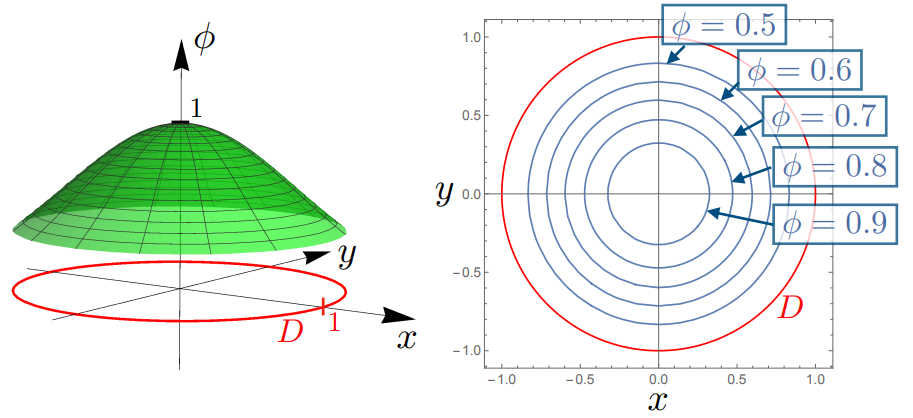
Fig. 3.1 Left Pane: An example of a two-dimensional scalar field, \(\phi(x,\, y) = \exp(-(x^2+y^2))\) (plotted in green on the \(z\) axis) defined over the domain \(D\,:\,x^2 + y^2 \leq 1\) (shown in red on the \((x,\,y)\) plane), Right Pane: Contour lines of the scalar field, showing lines of constant \(\phi\) in blue, within the domain \(D\).

3.2. Vector Fields

A vector field A scalar field is a physical quantity which has both magnitude and direction, at every point \({\bf r} = (x, \,y, \,z)\) within a domain. Physical examples include velocity, force, electric field and magnetic field. Mathematically we can write this as a function \(\bf A(r)\) such that:

\[\begin{split}{\bf A(r)} = \begin{pmatrix} A_x \,({\bf r})\\ A_y \,({\bf r})\\ A_z \,({\bf r}) \end{pmatrix}\end{split}\]

We can picture vector fields in Fig. 3.2, outlining a vector field

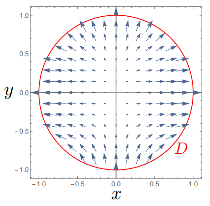
Fig. 3.2 The vector field \(\displaystyle {\bf A(r)} = \frac{1}{10}\begin{pmatrix} x\\ y^2 \end{pmatrix}\) over the domain \(D\,:\,x^2 + y^2 \leq 1\) (shown in red on the \((x,\,y)\) plane)

3.3. Calculus on Fields

Now that we have defined fields, which can vary according to different parameters at every point within a domain, we can begin to apply our toolkit of mathematical tools, here calculus.

We can find the partial derivatives of fields in a similar way to functions,

Worked example

Find the \(x,\, y\) derivatives for the fields:

\[\begin{split}\phi = \exp(-(x^2+y^2), \qquad {\bf A(r)} = \frac{1}{10}\begin{pmatrix} x\\ y^2 \end{pmatrix}\end{split}\]

\[\begin{split}\partial_x \phi &= -2x\,\exp(-(x^2+y^2) \\ \partial_y \phi &= -2y\,\exp(-(x^2+y^2) \\ \partial_x {\bf A(r)} &= \frac{1}{10}\begin{pmatrix} 1\\ 0 \end{pmatrix} \\ \partial_y {\bf A(r)} &= \frac{1}{10}\begin{pmatrix} 0\\ 2y \end{pmatrix} \end{split}\]

These partial derivatives measure the change of \(\phi\) along the directions of \(x\) or \(y\), but can we calculate the derivative of \(\phi\) along some general direction, characterised by a unit vector \(\hat{\bf u}\):

\[\begin{split}\hat{\bf u} = \begin{pmatrix} u_x\\ u_y\\ u_z \end{pmatrix} \end{split}\]

We need a directional derivative, which can tell us about the changes in \(\phi\) along each component of \(\hat{\bf u}\). This leads us to the gradient operator:

\[\begin{split}\nabla = \begin{pmatrix} \partial/\partial x \\ \partial/\partial y \\ \partial/\partial z \end{pmatrix} = \frac{\partial}{\partial x} \, \hat {\bf x} + \frac{\partial }{\partial y} \, \hat {\bf y}+ \frac{\partial}{\partial z} \, \hat {\bf z}\end{split}\]

which as an operator needs to act on a scalar field:

\[\begin{split}\nabla \phi = \begin{pmatrix} \partial\phi/\partial x \\ \partial\phi/\partial y \\ \partial\phi/\partial z \end{pmatrix} = \frac{\partial \phi}{\partial x} \, \hat {\bf x} + \frac{\partial \phi}{\partial y} \, \hat {\bf y}+ \frac{\partial \phi}{\partial z} \, \hat {\bf z}\end{split}\]

We see that this is now a vector field, which we can resolve in the \(\hat{\bf u}\) direction:

\[\hat{\bf u} \cdot \nabla \phi\]

which is our directional derivative of \(\phi\) in the \(\hat{\bf u}\) direction, which we often write as \(\nabla_{\hat{\bf u}} \phi\).

Looking at this expression further:

\[|\nabla_{\hat{\bf u}} \phi| = \hat{\bf u} \cdot \nabla \phi = |\hat{\bf u}||\nabla \phi|\cos (\theta) = |\nabla \phi|\cos (\theta)\]

• \(|\nabla_{\hat{\bf u}} \phi|\) is maximised when \(\theta = 0\) - The gradient \(\nabla \phi\) of a scalar field \(\phi\) always points toward the direction of maximum increase of \(\phi\) (i.e. a maxima).

• \(|\nabla_{\hat{\bf u}} \phi|\) is zero when \(\theta = \pi/2\), i.e. tangential surfaces, which would be given by \(\phi({\bf r}) = \text{constant}\) - this is always therefore one dimension lower than the dimension of the problem (therefore in 3D these would be surface areas and in 2D they would be contour lines).

We can always take some surface \(z = z(x,\,y)\) and convert it into a scalar field \(\phi\) with some surface normal \({\bf n} = \nabla \phi\).

Worked example

Consider \(\phi = \exp(-(x^2+y^2)\) defined over the domain \(x^2 + y^2 \leq 1\), find \(\nabla \phi\).

\[\begin{split}\nabla \phi = \begin{pmatrix} -2x\,\exp(-(x^2+y^2) \\ -2y\,\exp(-(x^2+y^2) \end{pmatrix} = -2\,\exp(-(x^2+y^2) \begin{pmatrix} x \\ y \end{pmatrix}\end{split}\]

We see that for all \(x,\, y\) within the domain, the vector will be directed inwards, as we see in Fig. 3.3.

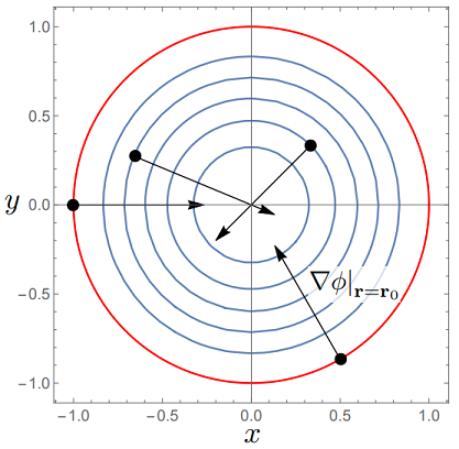
Fig. 3.3 Gradients \(\nabla \phi\) for a scalar field \(\phi({\bf r}) = \exp(-(x^2+y^2))\) at a few different points along the contour plot (denoted \(\bf r=r_0\)). The gradients are perpendicular to the contour lines and point toward the direction of the largest increase of \(\phi\), which from the surface plot in Fig. 3.1 we know is a maxima.

The gradient of \(\phi(x,\,y,\,z)\) will therefore be perpendicular to the surface \(\phi=c\), and we can use this to find the tangent plane to the surface at a given point.

Further worked examples

1. Find the gradient of the function \(f(x,\,y,\,z) = xyz\) at the point \((−2,\,3,\,4)\) and find the directional derivative of this function in the direction \({\bf v} = (3, \,-4, \,12)\).

We can find \(\nabla f\):

\[\begin{split}\nabla f = \begin{pmatrix}yz \\ xz \\ xy\end{pmatrix} \Rightarrow \nabla f\Bigg|_{(−2,\,3,\,4)} = \begin{pmatrix} 12 \\ -8 \\ -6\end{pmatrix}\end{split}\]

and therefore the directional derivative is given by:

\[\begin{split}\frac{1}{|{\bf v}|}{\bf v} \cdot \nabla f\Bigg|_{(−2,\,3,\,4)} \Rightarrow \frac{1}{\sqrt{3^2 + 4^2 + 12^2}} \begin{pmatrix} 3 \\ -4 \\ 12 \end{pmatrix}\cdot \begin{pmatrix} 12 \\ -8 \\ -6\end{pmatrix} = -\frac{4}{13}\end{split}\]

2. Find the tangent plane for the surface

\[z = x^3−y^3−2xy+2\]

at \(x=y=1\).

This equation means we can write \(\phi = x^3−y^3−2xy+2 - z = 0\) and therefore:

\[\begin{split}{\bf n} = \nabla \phi = \begin{pmatrix} 3x^2 - 2y \\ -3y^2 - 2x \\ -1 \end{pmatrix}\end{split}\]

The gradient of \(z = z(x,\,y)\) will be perpendicular to the contours of \(z\), projected in the \((x,\,y)\) plane, as illustrated in Fig. 3.4.

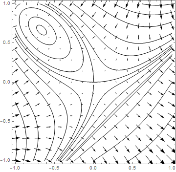
Fig. 3.4 A contour plot of the surface \(z = x^3−y^3−2xy+2\), together with the gradient field given by \(\nabla \phi = (3x^2−2y,\,−3y^2−2x,\,-1)\).

We can see that the gradient field vectors map out the stationary points on the function.

If we want to find the equation of the resulting tangent surface at a \(x=y=1\) we find \(z = 0\):

\[A:(1,\,1,\,0)\]

then we know that the scalar form of the tangent plane, which must satisfy \({\bf n}\cdot ({\bf r}- {\bf r_0}) = 0\) means:

\[\begin{split}{\bf n}|_A &= \begin{pmatrix} 3-2\\-3-2\\-1 \end{pmatrix} = \begin{pmatrix} 1\\-5\\-1 \end{pmatrix} \\ {\bf n}\cdot ({\bf r}- {\bf r_0}) = 0 &\Rightarrow \begin{pmatrix} 1\\-5\\-1 \end{pmatrix} \cdot\begin{pmatrix} x-1\\y-1\\z-0 \end{pmatrix} = 0 \\ &\Rightarrow x - 5y - z =-4\end{split}\]

3.4. Total Differential

Recall from our discussions about partial derivatives, we can also define a scalar total differential for a scalar field \(\phi(x,\,y,\,z)\):

\[\mathrm{d}\phi(x,\,y,\,z) = \frac{\partial \phi}{\partial x} \mathrm{d} x + \frac{\partial \phi}{\partial y} \mathrm{d} y + \frac{\partial \phi}{\partial z} \mathrm{d} z\]

which measures the infinitesimal change of \(\phi\) as we change \(x, \,y,\,z\) by infinitesimal amounts \(\mathrm{d}x, \,\mathrm{d}y,\, \mathrm{d}z\).
Likewise we can can the vectorial line element:

\[\begin{split}\mathrm{d}{\bf r} = \begin{pmatrix} \mathrm{d}x \\\mathrm{d}y\\ \mathrm{d}z\end{pmatrix} = \hat{\bf x}\, \mathrm{d}x + \hat{\bf y}\, \mathrm{d}y + \hat{\bf z} \, \mathrm{d}z \end{split}\]

to write the total differential in a slightly more compact notation:

\[\mathrm{d}\phi = \nabla \phi \cdot \mathrm{d}{\bf r}\]

To find the vector total differential, we can just use the multi-variate chain rule expression for a vectorised variable:

\[\mathrm{d}{\bf A}(x,\,y,\,z) = \frac{\partial {\bf A} }{\partial x} \mathrm{d} x + \frac{\partial {\bf A} }{\partial y} \mathrm{d} y + \frac{\partial {\bf A} }{\partial z} \mathrm{d} z\]

3.5. Different coordinate systems

The gradient operator does not need to be specified in Cartesian coordinates, we can also look at it in other coordinate systems too.

Using the result \(\mathrm{d}\phi = \nabla \phi \cdot \mathrm{d}{\bf r}\), we can examine the change in \(\mathrm{d}{\bf r}\) over different systems of coordinates, which will tell us how \(\nabla \phi\) will be different.

3.5.1. Cylindrical polar coordinates

Here the vectorial line element has the form:

\[\mathrm{d}{\bf r} = \hat{\bf r}\, \mathrm{d}r + \hat{\bf \theta }\,r\,\mathrm{d}\theta + \hat{\bf z} \,\mathrm{d}z\]

and looking at what we expect to get \(\mathrm{d}\phi\) from the multi-variate chain rule:

\[\mathrm{d}f = \frac{\partial f}{\partial r} \mathrm{d} r + \frac{\partial f}{\partial \theta} \mathrm{d} \theta + \frac{\partial f}{\partial z} \mathrm{d} z\]

then our expression for and so for \(\mathrm{d}\phi = \nabla \phi \cdot \mathrm{d}{\bf r}\) to match, we must have a gradient operator to be of the form:

\[\nabla f = \hat{\bf r}\, \frac{\partial f}{\partial r} + \hat{\bf \theta }\,\frac{1}{r}\,\frac{\partial f}{\partial \theta} + \hat{\bf z} \,\frac{\partial f}{\partial z} \]

3.5.2. Spherical polar coordinates

Here the vectorial line element has the form:

\[\mathrm{d}{\bf r} = \hat{\bf r} \,\mathrm{d}r + \hat{\bf \phi}\,r\,\mathrm{d}\phi + \hat{\bf \theta} \,r\,\sin(\phi)\,\mathrm{d}\theta\]

and looking at what we expect to get \(\mathrm{d}\phi\) from the multi-variate chain rule:

\[\mathrm{d}f = \frac{\partial f}{\partial r} \mathrm{d} r + \frac{\partial f}{\partial \phi} \mathrm{d} \phi + \frac{\partial f}{\partial \theta} \mathrm{d} \theta\]

then our expression for and so for \(\mathrm{d}\phi = \nabla \phi \cdot \mathrm{d}{\bf r}\) to match, we must have a gradient operator to be of the form:

\[\nabla f = \hat{\bf r}\, \frac{\partial f}{\partial r} + \hat{\bf \phi}\,\frac{1}{r}\,\frac{\partial f}{\partial \phi} + \hat{\bf \theta} \,\frac{1}{r\sin(\phi)}\,\frac{\partial f}{\partial \theta} \]

A very good resource for all these expressions can be found at Del in cylindrical and spherical coordinates