1. Coordinate Systems

1.1. Cartesian Coordinates (2D)

We can being by thinking about a 2D system of Cartesian coordinates, as illustrated in Fig. 1.1.

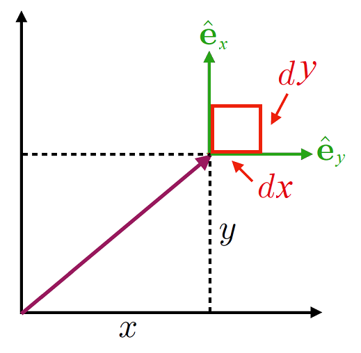
Fig. 1.1 A set of 2D Cartesian coordinate axes.

The standard ideas of presenting Cartesian coodinates as along the corridor and up the stairs apply, with \((x,\, y)\) or in terms of a vector:

\[\begin{split}{\bf r} = \begin{pmatrix} x\\ y\end{pmatrix}\end{split}\]

These coordinates can take any real value within \(x \in (\infty,\, \infty), \,y \in (\infty,\, \infty)\)

We can also find the infinitesimal changes in a Cartesian vector:

\[\begin{split}\mathrm{d}{\bf r} = \begin{pmatrix} \mathrm{d}x \\ \mathrm{d}y \end{pmatrix}\end{split}\]

and therefore the area element \(\mathrm{d}A\) is given by:

\[\mathrm{d}A = \mathrm{d}x\,\mathrm{d}y\]

1.2. Polar Coordinates (2D)

We can switch over from 2D Cartesian coordinates to a system of polar coordinates, as shown in Fig. 1.2

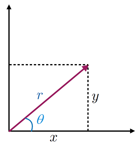
Fig. 1.2 A mapping between 2D Cartesian coordinates and 2D polar coordinates. Notice we switch from \((x,\,y) \rightarrow (r,\, \theta)\) coordinates, but always preserve having two pieces of information.

With coordinate transforms given by:

\[\begin{split}x &= r \cos(\theta) &\quad& r^2 = x^2 + y^2 \\ y &= r \sin(\theta) &\quad& \tan(\theta) = \frac{y}{x}\end{split}\]

We can see that the coordinates ranges here are \(r \in [0,\, \infty)\) and \(\theta \in [0,\,2\pi)\), although sometimes the range \(\theta \in (-\pi,\,\pi]\) is used instead.

In doing so we can rewrite the coordinate vector and find the infinitesimal changes:

\[\begin{split}{\bf r} &= \begin{pmatrix} r \cos(\theta) \\ r \sin(\theta) \end{pmatrix} \\ \Rightarrow \mathrm{d}{\bf r} &= \begin{pmatrix} \mathrm{d}r \cos(\theta) - r \sin(\theta)\mathrm{d}\theta \\ \mathrm{d}r \sin(\theta) + r \cos(\theta) \mathrm{d}\theta \end{pmatrix}\\ &= \begin{pmatrix} \cos(\theta) \\ \sin(\theta)\end{pmatrix}\mathrm{d}r + \begin{pmatrix} -\sin(\theta) \\ \cos(\theta) \end{pmatrix}r\mathrm{d}\theta\\ &= \hat{\bf r} \mathrm{d}r + \hat{\bf \theta} \mathrm{d}\theta\end{split}\]

where we have defined vectors for the \(r,\,\theta\) directions.

We notice here that these are actually unit vectors:

\[\begin{split}|\hat{\bf r}|^2 &= \cos^2(\theta) + \sin^2(\theta) = 1 \\ |\hat{\bf \theta}|^2 &= (-\sin(\theta))^2 + \cos^2(\theta) = 1\end{split}\]

and they are also orthogonal (perpendicular):

\[\hat{\bf r} \cdot \hat{\bf \theta} = -\cos(\theta)\,\sin(\theta) + \sin(\theta)\,\cos(\theta) = 0\]

So 2D polar coordinates actually make up an orthonormal coordinate basis (orthongoal and normalised)

We can see these illustrated in Fig. 1.3, where the \(\hat{\bf r},\, \hat{\bf \theta}\) coordinates can we see to be perpendicular and from the definition we see that that they staisfy all the properties of Equation (1.1).

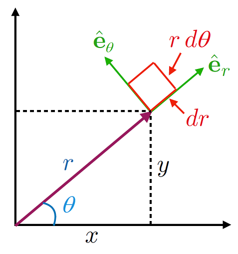
Fig. 1.3 Switching from Cartesian coordinate vectors to polar coordinate vectors.

and therefore the area element \(\mathrm{d}A\) is given by:

\[\mathrm{d}A = \left(\mathrm{d}r\right)\,\left(r\,\mathrm{d}\theta \right) = r\,\mathrm{d}r\,\mathrm{d}\theta\]

1.3. Cartesian Coordinates (3D)

In our discussion of vectors, we looked at the Cartesian coordinate system, which we can define in 3D using a system of basis vectors and the diagram in Fig. 1.4 to indicate the right handed axis convention.

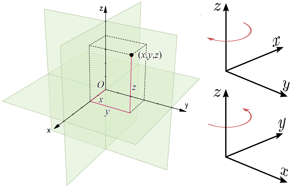
Fig. 1.4 Left: A set of 3D right handed Cartesian coordinate axes. Right: Upper figure left handed coordainte axes, Lower figure right handed coordinate axes.

Here we see that the coordindates can take any value in \(x \in (\infty,\, \infty), \,y \in (\infty,\, \infty),\, z \in (\infty,\, \infty)\)

We can write any vector in 3D as:

\[\begin{split}{\bf v} &= v_x\begin{pmatrix} 1 \\ 0 \\ 0 \end{pmatrix} + v_y\begin{pmatrix} 0 \\ 1 \\ 0 \end{pmatrix} + v_z\begin{pmatrix} 0 \\ 0 \\ 1 \end{pmatrix}\\ &= v_x\hat{\bf x} + v_y\hat{\bf y} + v_z\hat{\bf z}\end{split}\]

where we have clarified the basis vectors. Note that these satisfy the following properties;:

(1.1)\[\begin{split}|\hat{\bf x }| &= |\hat{\bf y }| = |\hat{\bf z }| = 1\\ \hat{\bf x} \cdot \hat{\bf y} &= \hat{\bf x} \cdot \hat{\bf y} = \hat{\bf x} \cdot \hat{\bf y} = 0 \\ \hat{\bf x} \times \hat{\bf y} &= \hat{\bf z} \\ \hat{\bf y} \times \hat{\bf z} &= \hat{\bf x} \\ \hat{\bf z} \times \hat{\bf x} &= \hat{\bf y} \end{split}\]

Another way to represent this is using a coordinate vector \({\bf r}\):

\[\begin{split}{\bf r} = \begin{pmatrix} x \\ y \\ z \end{pmatrix}\end{split}\]

which means we can look at the infinitesimal changes \(\mathrm{d}{\bf r}\):

\[\begin{split}{\bf r} = \begin{pmatrix} \mathrm{d}x \\ \mathrm{d}y \\ \mathrm{d} z \end{pmatrix}\end{split}\]

and therefore the volume element \(\mathrm{d}V\) is given by:

\[\mathrm{d}V = \mathrm{d}x\,\mathrm{d}y\,\mathrm{d}z\]

1.4. Spherical Polar Coordinates (3D)

In three dimensions, we can continute a switch to polar coordinates, with one length \(r\) and two angles \(\theta,\, \phi\) describing the three spatial dimensions \(x,\,y,\ z\):

\[\begin{split}x &= r \cos(\theta)\sin(\phi) \\ y &= r \sin(\theta)\sin(\phi) \\ z &= r \cos(\phi)\end{split}\]

which we see illustrated in Fig. 1.5.

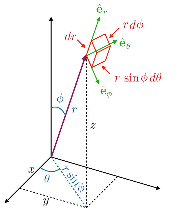
Fig. 1.5 One set of spherical polar axes, where the angle \(\phi\) denotes the declination from the \(z\) axes, this is called the Polar angle, this then leads to a projection on to the \(x-y\) plane \(r\sin(\phi)\). Then with the polar coordinates \(r,\, \theta\), known as the Radial and Azimuthal components (respectively), we further project on to the \(x,\,y\) axes.

We can then write the infinitesimal changes in the coordinate vector \(\bf r\) as:

\[\begin{split}{\bf r} &= \begin{pmatrix} r \cos(\theta)\sin(\phi) \\r \sin(\theta)\sin(\phi) \\ r \cos(\phi) \end{pmatrix} \\ \Rightarrow \mathrm{d}{\bf r} &= \begin{pmatrix} \mathrm{d}r \cos(\theta)\sin(\phi) - r \sin(\theta)\sin(\phi) \mathrm{d}\theta + r \cos(\theta)\cos(\phi) \mathrm{d}\phi\\ \mathrm{d}r \sin(\theta)\sin(\phi) + r \cos(\theta)\sin(\phi) \mathrm{d}\theta + r \sin(\theta) \cos(\phi)\mathrm{d}\phi \\ \mathrm{d}r \cos(\phi) - r \sin(\phi)\mathrm{d}\phi \end{pmatrix} \\ &= \begin{pmatrix} \cos(\theta)\sin(\phi) \\ \sin(\theta)\sin(\phi) \\ \cos(\phi) \end{pmatrix} \mathrm{d}r + \begin{pmatrix} \cos(\theta)\cos(\phi) \\ \sin(\theta) \cos(\phi)\\ - \sin(\phi) \end{pmatrix}r\mathrm{d}\phi + \begin{pmatrix} -\sin(\theta) \\ \cos(\theta)\\ 0\end{pmatrix} r\sin(\phi)\mathrm{d}\theta \\ &= \hat{\bf r} \,\mathrm{d}r + \hat{\bf \phi}\,r\,\mathrm{d}\phi + \hat{\bf \theta} \,r\,\sin(\phi)\,\mathrm{d}\theta\end{split}\]

and once again notice these are unit vectors:

\[\begin{split}|\hat{\bf r}|^2 &= \sin^2(\phi)\left(\cos^2(\theta) + \sin^2(\theta)\right) + \cos^2(\phi) = \sin^2(\phi) + \cos^2(\phi)= 1 \\ |\hat{\bf \phi}|^2 &= \cos^2(\phi)\left(\cos^2(\theta) + \sin^2(\theta)\right) + \sin^2(\phi) = \cos^2(\phi) + \sin^2(\phi)= 1 \\ |\hat{\bf \theta}|^2 &= (-\sin(\theta))^2 + \cos^2(\theta) = 1 \end{split}\]

and they are also orthogonal (perpendicular):

\[\hat{\bf r} \cdot \hat{\bf \phi} = \hat{\bf r} \cdot \hat{\bf \theta} = \hat{\bf \phi} \cdot \hat{\bf \theta} = 0\]

so spherical polar coordinates also form an orthonormal coordinate basis.

Each coordinate here has a range, \(r \in [0,\, \infty)\), whereas the two angles here have \(\theta \in [0,\, 2\pi),\, \phi \in [0,\, \pi)\). It might be a little confusing why the angles do not both go to \(2\pi\), however if we think about the going form \(\phi = 0 \rightarrow \phi = \pi\) this will form a semicircle. Rotating this around \(\theta = 0\rightarrow \theta = 2\pi\) does give a full sphere - so only one of the two spherical angles should be up to \(\pi\) and the other up to \(2\pi\).

In this convention, the volume element \(\mathrm{d}V\) is given by:

\[\mathrm{d}V = r^2\,\mathrm{d}r\,\sin(\phi)\,\mathrm{d}\phi\,\mathrm{d}\theta\]

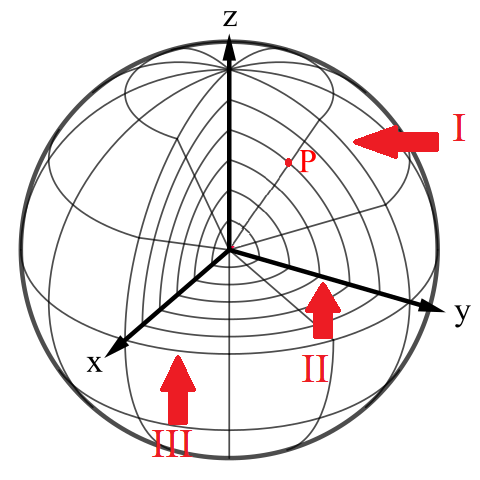
Fig. 1.6 A set of isobars for a spherical polar coordinate system,

We can see in Fig. 1.6 lines of constant \(r,\, \theta\) traced out along contour I, lines of constant \(\theta,\,\phi\) along contour II and lines of constant \(r,\, \phi\) along contour III. These are usually called isobars in some contexts and level surfaces or level curves in other contexts.

We might imagine that both \(\theta\) and \(\phi\) should go to \(2\pi\) here, but if we consider first going from pole to pole (i.e. with increasing \(\phi\)), this would trace out a semi-circle, which when rotated around the equator (i.e. increasing \(\theta\)) will trace out a full sphere.

This convention of angles is the one used most often in mathematics, although in physics a slightly different one is employed, as illustrated in Fig. 1.7. In this system the azimuthal angle is switched with the polar angle, but the physical intutition remains the same.

\[\begin{split}{\bf r} &= \begin{pmatrix} r \cos(\phi)\sin(\theta ) \\r \sin(\phi)\sin(\theta ) \\ r \cos(\theta ) \end{pmatrix} \\ \Rightarrow \mathrm{d}{\bf r} &= \begin{pmatrix} \mathrm{d}r \cos(\phi)\sin(\theta ) - r \sin(\phi)\sin(\theta ) \mathrm{d}\phi + r \cos(\phi)\cos(\theta ) \mathrm{d}\theta \\ \mathrm{d}r \sin(\phi)\sin(\theta ) + r \cos(\phi)\sin(\theta ) \mathrm{d}\phi + r \sin(\phi) \cos(\theta )\mathrm{d}\theta \\ \mathrm{d}r \cos(\theta ) - r \sin(\theta )\mathrm{d}\theta \end{pmatrix} \\ &= \begin{pmatrix} \cos(\phi)\sin(\theta ) \\ \sin(\phi)\sin(\theta ) \\ \cos(\theta ) \end{pmatrix} \mathrm{d}r + \begin{pmatrix} \cos(\phi)\cos(\theta ) \\ \sin(\phi) \cos(\theta )\\ - \sin(\theta ) \end{pmatrix}r\mathrm{d}\theta + \begin{pmatrix} -\sin(\phi) \\ \cos(\phi)\\ 0\end{pmatrix} r\sin(\theta )\mathrm{d}\phi \\x` &= \hat{\bf r} \mathrm{d}r + \hat{\bf \theta }r\mathrm{d}\theta + \hat{\bf \phi} r\sin(\theta )\mathrm{d}\phi\end{split}\]

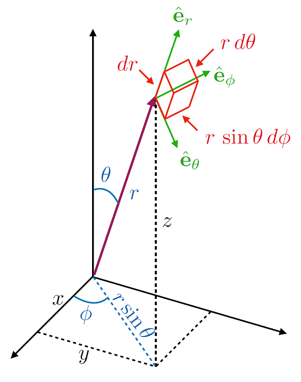
Fig. 1.7 Another set of spherical polar axes, where the angle \(\theta\) denotes the declination from the \(z\) axes, this then leads to a projection on to the \(x-y\) plane which then projects this further as per the polar coordinates \(r,\, \phi\).

Therefore here we see that in this convention \(r \in [0,\, \infty),\, \phi \in [0,\, 2\pi),\, \theta \in [0,\, \pi)\).

In this convention the volume element \(\mathrm{d}V\) is given by:

\[\mathrm{d}V = r^2\,\mathrm{d}r\,\sin(\theta)\,\mathrm{d}\theta\,\mathrm{d}\phi\]

Notice that either form here has the polar angle appearing in the \(\sin\) term

1.5. Cylindrical Polar Coordinates (3D)

Sometimes it makes more sense to combine the rotation symmetry of polar coordinates with the rectilinear nature of 3D Cartesian coodiantes, which results in a cylindrical coordinate system. Thus was have coordinate transforms of the form:

\[\begin{split}x &= r \cos(\theta)\\ y &= r \sin(\theta)\\ z &= z\end{split}\]

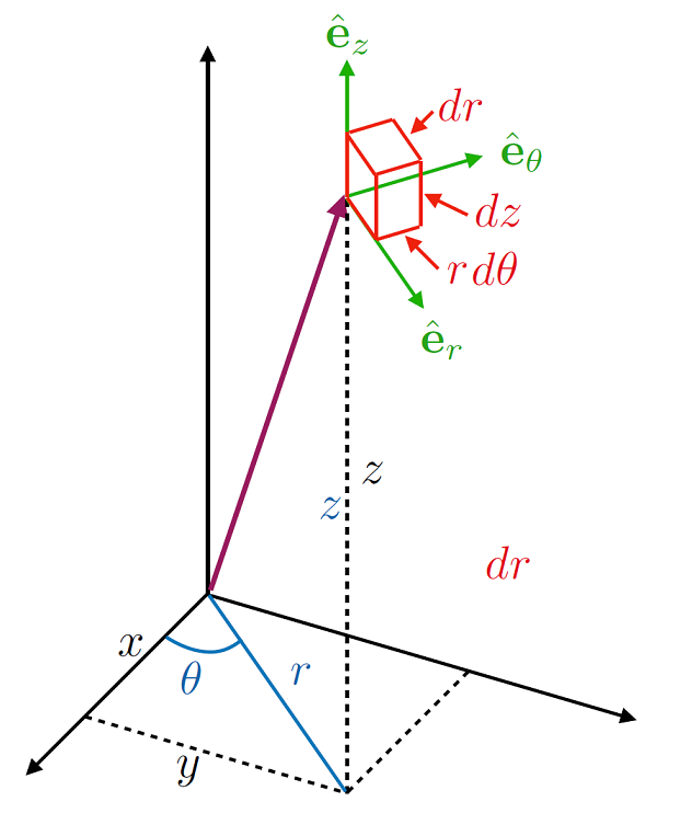
Fig. 1.8 One set of cylidrical polar axes, where the angle \(\theta\) is the polar angle around the \(z\) axis and distance \(r\) is in the \(x-y\) plane, with the elevation from the plane determined by \(z\).

Here \(r \in [0,\, \infty),\, \theta \in [0,\, 2\pi),\, z \in (-\infty,\, \infty)\). Notice that in contrast to the spherical polar coordinate system, the radial vector \(r\) is only the distance in the \(x-y\) plane. Sometimes this system is written in terms of \((\rho, \,\phi,\, z)\), but this is just a variable relabelling.

To find the infinitesimal changes in the coordinates here we find:

\[\begin{split}{\bf r} &= \begin{pmatrix} r \cos(\theta) \\r \sin(\theta) \\ z \end{pmatrix} \\ \Rightarrow \mathrm{d}{\bf r} &= \begin{pmatrix} \mathrm{d}r \cos(\theta) - r \sin(\theta) \mathrm{d}\theta \\ \mathrm{d}r \sin(\theta) + r \cos(\theta) \mathrm{d}\theta \\ \mathrm{d}z \end{pmatrix} \\ &= \begin{pmatrix} \cos(\theta) \\ \sin(\theta) \\ 0 \end{pmatrix} \mathrm{d}r + \begin{pmatrix} -\sin(\theta) \\ \cos(\theta)\\ 0 \end{pmatrix}r\mathrm{d}\theta + \begin{pmatrix} 0 \\ 0\\ 1\end{pmatrix}\mathrm{d}z \\ &= \hat{\bf r} \mathrm{d}r + \hat{\bf \theta }r\mathrm{d}\theta + \hat{\bf z} \mathrm{d}z\end{split}\]

and therefore the volume element \(\mathrm{d}V\) is given by:

\[\mathrm{d}V = r\,\mathrm{d}r\,\mathrm{d}\theta\,\mathrm{d}z\]