2. Multidimensional Integrals

Although we are used to find the area under a curve from the integral of a function \(f(x)\) over some limits \(x \in [a,\, b]\):

\[A = \int_a^b f(x)\,\mathrm{d}x\]

we could think about area of a space a difference way. Suppose we had a revion described by some boundary function \(B(x,\,y)\), as depicted in Fig. 2.1:

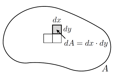
Fig. 2.1 Division of a 2-dimensional area A into infinitesimal area elements \(\mathrm{d}A\).

The easiest way to calculate the area here would be break up the space into infinitesimal building blocks of size \(\mathrm{d}A = \mathrm{d}x\,\mathrm{d}y\). Then all that we would need to do is perform the integration in the relevant region - i.e. the limits of the integration are quite important. Conceptually we can think of \(\mathrm{d}A\) just like we do for the one variable case of integration, breaking up a shape into infintesimal blocks which we then sum up over the integral,

Likewise if we had some scalar which has values at all points in space, described by a function \(f(x,\,y)\), then we could try to find the how the area contained within the bounded shape has a weighting at each point due to \(f(x,\,y)\). Likewise if we have some function \(f(x,\,y,\,z)\) describing some shape in 3D space,. We can think of these as multidimensional integals as extending integral calculus to multi-dimensions, akin to partial differentiation extending differential calculus to multi-varibles.

2.1. Area Integrals

Definition

Formally we can think of the area in some space that we define through the relevant limits:

\[A = \iint_{area}\,\mathrm{d}A = \int_{a(x,\,y)}^{b(x,\,y)}\,\mathrm{d}x\,\int_{c(x,\,y)}^{d(x,\,y)}\mathrm{d}y\]

The caveat now being that these limits can vary with respect to the space also. This sort of area integral is known as a double integral, because we have to perform integrals over both the \(x\) and \(y\) variables. When integrating over one variable, the other is held constant - akin to how we do partial differentiation too.

This is just doing the integral as is, we could also introduce an intregrand:

\[I = \int_A \phi({\bf r})\,\mathrm{d}A = \iint_A\phi({\bf r})\,\mathrm{d}x\,\mathrm{d}y\]

where we have some function - which is often called a scalar field \(\phi(x,\,y) = \phi({\bf r})\) which has as inputs \(\bf r = (x,\, y)\), some 2D position vector. We note therefore that an important special case is \(\phi = 1\), where the area integral is equal to the total area, \(A = \iint_A \,\mathrm{d}A\). Otherwise what we are finding is an area weighed by the function \(\phi\).

The order of the integration can however sometimes matter - this becomes important if the limits of each of the integals depends on one of the other variables (this can happen as when the integration is done, all the other variables are considered constant).

Worked example

Lets think about a flat 2D sheet with some density \(\sigma(x,\,y)\) (mass per unit area), as depcited in Fig. 2.2,

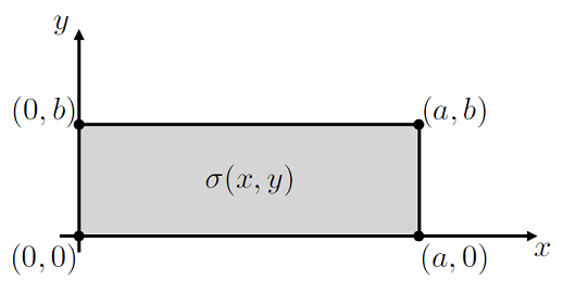
Fig. 2.2 Rectangular plate with some density \(\sigma(x,\,y)\).

To find the area of the plate we can perform a double integral, knowing that there are boundaries at \(x \in [0,\,a]\) and \(y \in [0,\,b]\):

\[A = \iint_A\,\mathrm{d}A =\int_0^a\,\mathrm{d}x\,\int_0^b\,\mathrm{d}y = \Big[ x\Big]_{0}^a \Big[ y\Big]_0^b = ab\]

The total mass of the plate will be given by an integral weighted by the density function:

\[M = \iint_A\sigma(\bf{r})\,\mathrm{d}A = \int_0^a\,\int_0^b\,\sigma(x,\,y)\,\mathrm{d}x\,\mathrm{d}y = \int_0^a\,\mathrm{d}x\,\int_0^b\,\mathrm{d}y\,\sigma(x,\,y)\]

where we use the final notation for brevity and ease of expression - it does not mean not to include the \(\sigma\) term in the evaluation of the integrals.

If the rectangular plate has a uniform density, then \(\sigma\) is just a constant and we find:

\[M = \sigma\,\int_0^a\,\mathrm{d}x\,\int_0^b\,\mathrm{d}y = \sigma\,a\,b = \sigma \,A\]

If the rectangular plate has a uniform density, then we need to evaluate the integrals in turn,

e.g. for \(\sigma(x,\, y) = y^2 + xy\), we can calculate the \(y\) integral first:

\[M = \int_0^a\,\mathrm{d}x\,\int_0^b\,\mathrm{d}y\,(y^2 + xy) = \int_0^a\,\Bigg[\frac{1}{2}xy^2 + \frac{1}{3}y^3\Bigg]_0^b\,\mathrm{d}x = \int_0^a\,\left(\frac{1}{2}x b^2 + \frac{1}{3}b^3\right)\,\mathrm{d}x\]

This is now reduced the 2D integral to a 1D integral, which we can evaluate:

\[M = \left[\frac{1}{4}x^2 b^2 + \frac{1}{3}b^3x\right]_0^a = \frac{1}{4}a^2b^2 + \frac{1}{3}ab^3\]

If we reverse the order integration however, starting from the \(x\) integral, we find:

\[\begin{split}M &= \int_0^a\,\mathrm{d}x\,\int_0^b\,\mathrm{d}y\,(y^2 + xy) = \int_0^b\,\Bigg[\frac{1}{2}x^2y + xy^2\Bigg]_0^a\,\mathrm{d}y = \int_0^a\,\left(\frac{1}{2}y a^2 + ay^2\right)\,\mathrm{d}y \\ &= \left[\frac{1}{4}y^2 a^2 + \frac{1}{3}ay^3\right]_0^a = \frac{1}{4}a^2b^2 + \frac{1}{3}ab^3\end{split}\]

So we see in this case, the order of integration does not matter.

2.1.1. Non-constant limits

Sometimes however we have to deal with boundaries that are not constant (at least in the coordinate system, e.g. a circular arc can be described with constant in polar coordinates, but the Cartesian coordinates would be varying).

Think about a straight line boundary but now one at an angle, as depicted in Fig. 2.3.

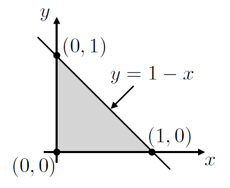
Fig. 2.3 Triangular area bounded by coodinate axes as well as linear function \(y = 1-x\).

We see here that the limits of the two integrals cannot both be constant - upper limit of the \(y\) integral will change depending on the value of \(x\) (or vice-versa), hence we need limits of the form \(x \in[0,\, 1]\) and \(y \in [0,\, 1-x]\). This makes the double integral take the form:

\[A = \int_0^1\,\mathrm{d}x\,\int_0^{1-x}\,\mathrm{d}y\]

Now that there is some function of \(x\) in the limit, this says evaluate the \(y\) integral first and the \(x\) integral last:

\[A = \int_0^1\,\mathrm{d}x\,\Big[y\Big]_0^{1-x} = \int_0^1(1-x)\,\mathrm{d}x = \left[x - \frac{1}{2}x^2\right]_0^1 = \frac{1}{2}\]

We can also switch round the integration, but choosing to have \(y \in [0,\, 1],\, x \in [0,\, 1-y]\), which means that:

\[\begin{split}A &= \int_0^1\,\mathrm{d}y\,\int_0^{1-y}\,\mathrm{d}x \\ &= \int_0^{1}\,\mathrm{d}y\,\Big[x\Big]_0^{1-y} = \int_0^1 (1-y)\,\mathrm{d}y = \left[y - \frac{1}{2}y^2\right]_0^1 = \frac{1}{2}\end{split}\]

So the order of the integration does matter in this example - if we did the \(x\) integral first, the final result would appear to depend on \(x\), which the area here clearly cannot.

In fact the choice of coordinates we choose will not change the value of the integral either, lets look at doing these sorts of integral in polar coordinates, given \(y^2 + x^2 = R^2\) for \(y \geq 0\), as depicted in Fig. 2.4:

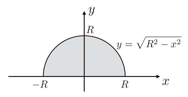
Fig. 2.4 Area shown as a shaded region composed of a half circle.

In Cartesian coordinates to find this area we have \(x \in [-R,\,R]\) but since

\[x^2 + y^2 = r^2 \Rightarrow y = \pm \sqrt{R^2-x^2}\]

we would need to do:

\[A = \int_{-R}^R\,\mathrm{d}x\,\int_0^{\sqrt{R^2 -x^2}}\,\mathrm{d}y = \int_{-R}^R\sqrt{R^2 - x^2}\,\mathrm{d}x\]

which will then require an integral substitution to solve, quite a pain!

In polar coodinates this region is given by \(r \in [0,\,R]\) and \(\theta \in [0,\,\pi]\) and given that \(A = \iint\,r\mathrm{d}r\,\mathrm{d}\theta\) i polar coordiantes, we have to find:

\[A = \int_0^R\,r\mathrm{d}r\,\int_0^{\pi}\,\mathrm{d}\theta = \pi\left[\frac{1}{2}r^2\right]_0^\pi = \frac{1}{2}\pi R^2\]

giving the result we expect!

Further worked examples

1. Lets look a more involved example, \(f(x,\,y) = x^2 + 2xy\) and we are interested in an area over a triangle, as depicted in Fig. 2.3:

We see here that the limits of the two integrals cannot both be constant - upper limit of the \(y\) integral will change depending on the value of \(x\) (or vice-versa), hence \(x \in[0,\, 1]\) and \(y \in [0,\, 1-x]\) is one way to think about this area:

\[I_A = \iint f(x,\,y)\,\mathrm{d}A = \int_0^1\,\mathrm{d}x\,\int_0^{1-x}\,\mathrm{d}y\,(x^2 + 2xy)\]

Now that there is some function of \(x\) in the limit, this says evaluate the \(y\) integral first and the \(x\) integral last:

\[\begin{split}I_A &= \int_0^1\,\mathrm{d}x\,\Bigg[x^2y + xy^2\Bigg]_0^{1-x} = \int_0^1\,\mathrm{d}x\,\Bigg[x^2(1-x) + x(1-x)^2\Bigg] \\ &= \int_0^1\,\mathrm{d}x\,(x-x^2) = \Bigg[\frac{1}{2}x^2 - \frac{1}{3}x^3 \Bigg]_0^1 = \frac{1}{6}\end{split}\]

We can also switch round the integration, but choosing to have \(y \in [0,\, 1],\, x \in [0,\, 1-y]\), which means that:

\[\begin{split}I_A &= \int_0^{1-y}\,\mathrm{d}x\,\int_0^{1}\,\mathrm{d}y\,(x^2 + 2xy) = \int_0^1\,\mathrm{d}y\,\Bigg[\frac{1}{3}x^3 + x^2y\Bigg]_0^{1-y} \\ &= \int_0^1\,\mathrm{d}y\,\Bigg[\frac{1}{3}(1-y)^3 + y(1-y)^2\Bigg] = \int_0^1\,\mathrm{d}y\,\left(\frac{2}{3}y^3 - y^2 + \frac{1}{3}\right) \\ &= \Bigg[\frac{1}{6}y^4 - \frac{1}{3}y^3 +\frac{1}{3}y\Bigg]_0^1 = \frac{1}{6}\end{split}\]

2. This looks at a trickier set of limits, lets try and calculate the integral \(I_A = \iint_A x^2y\,\mathrm{d}A\) for an area composed of a rectangle and a semi-circle, as depicted in Fig. 2.5:

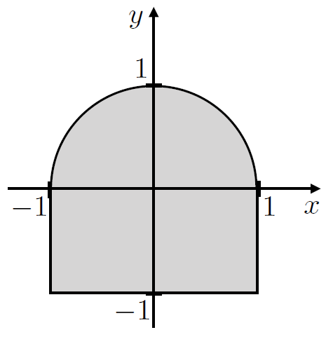
Fig. 2.5 Area shown as a shaded region composed of a rectangle and a half circle.

If we pick \(x \in [-1,\,1]\), then the \(y\) limits for the two integrals would be from the lower limit \(y = -1\) to the coorsiante axes \(y = 0\) and from the coordinate axes \(y = 0\) up to the upper limit at the semi-circle edge \(y = \sqrt{R^2-x^2}\). So this becomes:

\[I_A = \int_{-1}^1 \,\mathrm{d}x\,\Bigg[\int_{-1}^{0}\,\mathrm{d}y + \int_{0}^{\sqrt{1-x^2}}\,\mathrm{d}y \Bigg]x^2y\]

Since the two \(y\) integral terms will add together we could write them as one integral over \(y \in [-1,\, \sqrt{1-x^2}]\), so the area is found by:

\[\begin{split}I_A &= \int_{-1}^1 \,\mathrm{d}x\,\int_{-1}^{\sqrt{1-x^2}}x^2y\,\mathrm{d}y = \int_{-1}^1\Bigg[\frac{1}{2}x^2y^2\Bigg]_{-1}^{\sqrt{1-x^2}} \,\mathrm{d}x\\ &= \frac{1}{2}\int_{-1}^1\left(x^2(1-x^2) - x^2\right) \,\mathrm{d}x = -\frac{1}{2}\int_{-1}^1 x^4\,\mathrm{d}x = -\frac{1}{5}\end{split}\]

We could do this integral the other way round, but this is quite a bit tricker!

2.2. Volume Integrals

The concept of an area integral can be extended to volume integrals, moving from a 2D space with a double integral to a 3D space with a triple integal.

Defintion

The integration region is divided up into volume elements \(\mathrm{d}V\), in Cartesian coordinates, the volume element is simply \(\mathrm{d}V = \mathrm{d}x\,\mathrm{d}y\,\mathrm{d}z\) as depicted in Fig. 2.6.

The volume can be expressed as a triple integral over \(x, \,y,\, z\):

\[V = \iiint_V \,\mathrm{d}V = \int_{a(x,\,y,\,z)}^{b(x,\,y,\,z)}\,\mathrm{d}x\,\int_{c(x,\,y,\,z)}^{d(x,\,y,\,z)}\,\mathrm{d}y\,\int_{e(x,\,y,\,z)}^{f(x,\,y,\,z)}\,\mathrm{d}z\]

where the integration limits can (in general) be non-constant in space depending on the surface region. Likewise we can use a scalar field \(\phi(x,\,y,\,z)\) as a weighting function here also, e.g. to calculate a total mass from a density function:

\[I_V = \iiint_V \phi(x,\,y,\,z)\,\mathrm{d}V\]

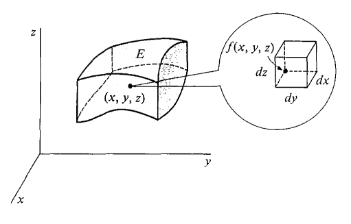
Fig. 2.6 A triple integral of a surface based on the infinitesimal building blocks of the volume, here in Cartesian coordinates \(\mathrm{d}V = \mathrm{d}x\,\mathrm{d}y\,\mathrm{d}x\).

2.2.1. Non-constant limits

We can try to find three dimensional equivalent of the wedge in Fig. 2.3, with a space bounded by the coorindate axes as well as the plane

\[x + y+ z = 1\]

This might look confusing, but if we looks at each of the \(x-y\), \(x-z\) and \(y-z\) planes we can see that this reduces to three lines:

\[\begin{split}z = 0 & \qquad x + y = 1 \Rightarrow y = 1-x\\ y = 0 & \qquad x + z = 1 \Rightarrow z = 1-x\\ x = 0 & \qquad y + z = 1 \Rightarrow z = 1-y\end{split}\]

this means that we can take our two dimensional result and add on additional non-constant limits:

\[V = \int_0^1\,\mathrm{d}x\,\int_0^{1-x}\,\mathrm{d}y\,\int_0^{1-x-y}\,\mathrm{d}z \]

which we can then evaluate:

\[\begin{split}V &= \int_0^1\,\mathrm{d}x\,\int_0^{1-x}\Big[z\Big]_0^{1-x-y}\,\mathrm{d}y\\ &= \int_0^1\,\mathrm{d}x\,\int_0^{1-x}\Big(1-x-y\Big)\,\mathrm{d}y = \int_0^1\Big[y-xy-\frac{1}{2}y^2\Big]_0^{1-x}\,\mathrm{d}x \\ &= \int_0^1\Big[(1-x)-x(1-x)-\frac{1}{2}(1-x)^2\Big]_0^{1-x}\,\mathrm{d}x \\ &= \int_0^1\Big((1-x)^2-\frac{1}{2}(1-x)^2\Big)\,\mathrm{d}x = \int_0^1\Big(\frac{1}{2}(1-x)^2\Big)\,\mathrm{d}x \\ &= \frac{1}{2}\int_0^1\Big(1-2x+x^2\Big)\,\mathrm{d}x = \frac{1}{2}\Big[x-x^2+\frac{1}{3}x^3\Big]_0^1 \\ &= \frac{1}{2}\Big(1-(1)^2+\frac{1}{3}(1)^3\Big) = \frac{1}{6}\\\end{split}\]

If we thought about this problem in terms of vectors, then we could have used the triple scalar product to find the area of a triangular pyramid:

\[\left|\frac{1}{6}\hat{\bf x}\cdot (\hat{\bf y}\times \hat{\bf z})\right| = \frac{1}{6}\]

2.2.2. Spherical polar coordinates

If we wanted to find the volume of a sphere of radius \(R\), we could calculate this using cartesian coordinates, where \(x \in [-R,\, R]\) and then akin to the circle area in 2D \(y \in[-\sqrt{R^2 - x^2},\,-\sqrt{R^2 - x^2}]\) and finally to elevate this to a volume in 3D \(z \in[-\sqrt{R^2 - x^2 - y^2},\,-\sqrt{R^2 - x^2 - y^2}]\)

\[V = \iiint\,\mathrm{d}V = \int_{-R}^R \,\mathrm{d}x\,\int_{-\sqrt{R^2 - x^2}}^{\sqrt{R^2 - x^2}}\, \mathrm{d}y\,\int_{-\sqrt{R^2 - x^2-y^2}}^{\sqrt{R^2 - x^2-y^2}} \,\mathrm{d}z\]

truely a nightmare to solve!

Instead lets switch to spherical polar coordinates, with \(r \in[0, \,R],\, \phi \in [0,\,\pi],\, \theta \in [0,\, 2\pi]\):

\[\begin{split}V &= \iiint\,\mathrm{d}V = \int_0^R r^2\,\mathrm{d}r\,\int_0^\pi\sin(\phi)\,\mathrm{d}\phi\,\int_0^{2\pi}\,\mathrm{d}\theta \\ &= 2(2\pi)\Bigg[\frac{1}{3}r^3\Bigg]_0^R = \frac{4}{3}\pi R^3\end{split}\]

as expected.

2.2.3. Cylindrical polar coordinates

We can find the volume of a cylinder with radius \(R\) and height \(H\) (recall this could be done through a solid of revolution type calculation, but here we aim to think about 3D axes), in Cartesian coordinates this would take the form of \(x \in [-R,\, R]\) then in 2D the circular cross section would be found through \(y \in [-\sqrt{R^2 - x^2},\,\sqrt{R^2 - x^2}]\) and then the height \(z \in [0,\, H]\), giving:

\[V = \iiint\,\mathrm{d}V = \int_{-R}^R \,\mathrm{d}y\,\int_{-\sqrt{R^2 - x^2}}^{\sqrt{R^2 - x^2}}\, \mathrm{d}y\,\int_{0}^{H} \,\mathrm{d}z\]

still not a great integral to compute, an integration variable change would be required.

In cylindrical polar coordinates however, \(r \in[0, R], \theta \in [0,\, 2\pi],\, z \in [0,\, H]\):

\[\begin{split}V &= \iiint\,\mathrm{d}V = \int_0^R r\,\mathrm{d}r\,\int_0^{2\pi}\,\mathrm{d}\theta\,\int_0^{H}\,\mathrm{d}z \\ &= 2\pi H \Bigg[\frac{1}{2}r^2\Bigg]_0^R = \pi R^2 H\end{split}\]

as expected.

Further worked examples

1. Calculate the triple integral of the function

\[f(x,\, y,\, z) = \frac{1}{2} \left(x^2 + y^2 + z^2\right)\]

over a cube whose corners are at the points \({\bf r} = (\pm 1,\, \pm 1,\, \pm 1)\):

\[\begin{split}I_V &= \int_{-1}^1\,\mathrm{d}x\,\int_{-1}^1\,\mathrm{d}y\,\int_{-1}^1\,\mathrm{d}z\, \left[\frac{1}{2} \left(x^2 + y^2 + z^2\right)\right]\\ &= \frac{1}{2}\int_{-1}^1\,\mathrm{d}x\,\int_{-1}^1\,\mathrm{d}y\,\Bigg[x^2z + y^2z +\frac{1}{3}z^3\Bigg]_{-1}^1\\ &= \int_{-1}^1\,\mathrm{d}x\,\int_{-1}^1\,\mathrm{d}y\,\Bigg(x^2 + y^2 +\frac{1}{3}\Bigg)= \int_{-1}^1\,\mathrm{d}x\,\Bigg[x^2y + \frac{1}{3}y^3 +\frac{1}{3}y\Bigg]_{-1}^1\\ &= 2\int_{-1}^1\,\mathrm{d}x\,\Bigg(x^2 + \frac{2}{3} \Bigg) = 2\Bigg[\frac{1}{3}x^3 +\frac{2}{3}x\Bigg]_{-1}^1 = 4\end{split}\]

2. Find the volume integral of the scalar field

\[f(x,\,y) = x^2y\]

over a tetrahedral volume, bounded by the \(x-y\), \(y-z\) and \(x-z\) axes as well as the surface \(x + y+ z = 1\), since all the bounding surfaces are symmetric in \(x,\, y,\, z\), there is no initial preference in integration order, however the integrand does not contain \(z\) so this is likely to be the easiest initial integral to compute, therefore:

\[I_V = \iiint\,\mathrm{d}V\,x^2y \]

with \(x = 0, \,y = 0,\, z = 0\) up to the plane \(x + y + z = 1\).

Therefore in the \(z\) plane the limits are \(z \in[0,\, 1 - x - y]\) and likewise in the \(y\) plane the limits would be \(y \in [0,\, 1-x]\) (since \(z=0\) along this plane), hence along with \(x \in[0,\, 1]\):

\[\begin{split}I_V &= \int_0^1\,\mathrm{d}x\,\int_0^{1-x}\,\mathrm{d}y\,\int_0^{1-x-y}x^2y\,\mathrm{d}z \\ &= \int_0^1\,\mathrm{d}x\,\int_0^{1-x}\,\mathrm{d}y\Bigg[x^2yz \Bigg]_0^{1-x-y} = \int_0^1\,\mathrm{d}x\,\int_0^{1-x}\,\mathrm{d}y\left(x^2y(1-x-y)\right)\\ &= \int_0^1\,\mathrm{d}x\,\int_0^{1-x}\left(x^2y-x^3y-x^2y^2\right)\,\mathrm{d}y\\ &= \int_0^1\,\mathrm{d}x\,\int_0^{1-x}\Bigg[\frac{1}{2}x^2y^2-\frac{1}{2}x^3y^2-\frac{1}{3}x^2y^3\Bigg]_0^{1-x}\\ &= \frac{1}{6}\int_0^1\left(x^2 - 3x^3 + 3x^4 - x^5\right)\,\mathrm{d}x \\ &= \frac{1}{6}\Bigg[\frac{1}{3}x^3 - \frac{3}{4}x^4 + \frac{3}{5}x^5 - \frac{1}{6}x^6\Bigg]_0^{1}= \frac{1}{360}\end{split}\]