7. Vector Calculus Theorems

Although the ideas in vector calculus seem quite distinct, area, surface and volume integrals as well as the gradient, divergence and curl, it turns out that they are connected together thanks to a couple of quite important theorems. These can in some cases simplify a calculation that we are aiming to do and/or give us a better intution about a system.

7.1. Gradient Theorem

Definition

The gradient theorem states that for a scalar field \(f({\bf r})\), we can use the multi-variable chain rule to show that:

\[\int_{\mathcal{C}} \nabla f\cdot \mathrm{d}{\bf r} = \int_{{\bf r} = a}^{{\bf r} = b} \,\mathrm{d}f = f(b) - f(a)\]

where the contour \(\mathcal{C}\) is defined over the points \(f(a) \rightarrow f(b)\).

This statement, which really just relies on multi-variable chain rule, also allows us to make the strong statement that for a conservative vector field, i.e. one where \({\bf F}({\bf r}) = \nabla \phi({\bf r})\) the line integral is path independent - we can see here it only depends on the starting/finishing points.

This is to be contrasting with a general vector field \({\bf F} = \nabla \phi + \nabla \times {\bf A}\), which clearly would be path dependent due to the curl term adding additional parts to the integral here.

7.2. (Gauss-)Divergence Theorem

Definition

The divergence theorem states that for a vector field \({\bf F}({\bf r})\), that is defined over a volume \(V\) with boundary surface area \(S\):

\[\iint_S {\bf F}({\bf r})\cdot \mathrm{d}{\bf S} = \iiint_V \left(\nabla \cdot F\right)\,\mathrm{d}V\]

For a volume \(V\) in space, this will be enclosed by some surface area \(S = \partial V\) (not to be confused with taking some partial derivative!), as depicted in Fig. 7.1.

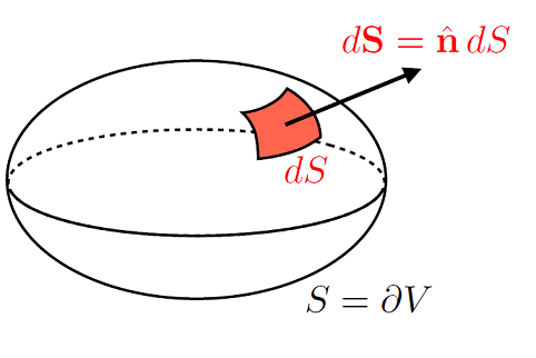
Fig. 7.1 Vectorial surface-area element \(\mathrm{d}{\bf A}\) of a closed surface \(S = \partial V\), with the convention that \(\mathrm{d}{\bf A} = \hat{\bf n} \mathrm{d}A\) points outwards.

Worked example

Consider the vector field:

\[\begin{split}{\bf F}({\bf r}) = \begin{pmatrix} x^2 \\ y \\ z \end{pmatrix}\end{split}\]

over a cubic volume surface, centered on the origin, with corners \((\pm 1,\, \pm 1,\, \pm 1)\).

In order to calculate the surface integral, we could need to find each of the surface normals for each face of the cube, as depicted in Fig. 7.2.

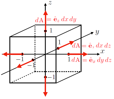
Fig. 7.2 A cubic volume with each surface normal indicated by a red arrow.

If we compute the surface integral, since the surfaces are over constant planes in each dimension, we don’t need to parameterise the integrals in this case:

\[\begin{split}&\iint_{S} {\bf F}({\bf r})\cdot \mathrm{d}{\bf A}= \\ & \int_{-1}^1 \,\mathrm{d}y\,\int_{-1}^1\,\mathrm{d}z \,\begin{pmatrix} 1^2 \\ y \\ z \end{pmatrix} \cdot \begin{pmatrix} 1 \\ 0 \\ 0 \end{pmatrix} + \int_{-1}^1 \,\mathrm{d}y\,\int_{-1}^1\,\mathrm{d}z \,\begin{pmatrix} (-1)^2 \\ y \\ z \end{pmatrix} \cdot \begin{pmatrix} -1 \\ 0\\ 0 \end{pmatrix} \\ &+ \, \int_{-1}^1 \,\mathrm{d}x\,\int_{-1}^1\,\mathrm{d}z \,\begin{pmatrix} x^2 \\ 1 \\ z \end{pmatrix} \cdot \begin{pmatrix} 0 \\ 1 \\ 0 \end{pmatrix} + \int_{-1}^1 \,\mathrm{d}x\,\int_{-1}^1\,\mathrm{d}z \,\begin{pmatrix} x^2 \\ -1 \\ z \end{pmatrix} \cdot \begin{pmatrix} 0 \\ -1 \\ 0 \end{pmatrix} \\ &+ \, \int_{-1}^1 \,\mathrm{d}x\,\int_{-1}^1\,\mathrm{d}y \,\begin{pmatrix} x^2 \\ y \\ 1 \end{pmatrix} \cdot \begin{pmatrix} 0 \\ 0 \\ 1 \end{pmatrix} + \int_{-1}^1 \,\mathrm{d}x\,\int_{-1}^1\,\mathrm{d}y \,\begin{pmatrix} x^2 \\ y \\ -1 \end{pmatrix} \cdot \begin{pmatrix} 0 \\ 0 \\ -1 \end{pmatrix} \\ &= \, \int_{-1}^1\,\int_{-1}^1 \,\Big( 1 - 1 \Big)\,\mathrm{d}y\,\mathrm{d}z + \int_{-1}^1 \,\int_{-1}^1\, \Big( 1 + 1 \Big)\,\mathrm{d}x\,\mathrm{d}z + \int_{-1}^1\,\int_{-1}^1 \, \Big( 1 + 1\Big)\,\mathrm{d}x\,\mathrm{d}y \\ &= 0 + 2(2)(2) + 2(2)(2) = 16\end{split}\]

A little long! However using the divergence theorem:

\[\begin{split}\nabla \cdot {\bf F} &= 2x + 2\\ \iint_S {\bf F}\cdot\mathrm{d}{\bf r} &= \iiint_{V} (\nabla \cdot {\bf F})\,\mathrm{d}V = \int_{-1}^1\,(2x + 2)\,\mathrm{d}x\, \int_{-1}^1\,\mathrm{d}y\, \int_{-1}^1\,\mathrm{d}z \\ &= (2)(2)\int_{-1}^1\,(2x+2)\,\mathrm{d}x = 4\Bigg[x^2 + 2x\Bigg]_{-1}^1 = 16\end{split}\]

In agreement with the previous result and whole lot easier to do!

7.2.1. A Sketch of a Proof

We can sketch out a proof of this result, using an infinitesimal volume cube \(\mathrm{d}V\) as depicted in Fig. 7.3.

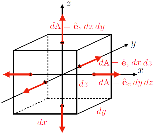
Fig. 7.3 An infinitesimal cubic surface \(\mathrm{d}V = \mathrm{d}x\,\mathrm{d}y\,\mathrm{d}z\) around some vector field divergence.

Thinking about an infinitesimal flux element \(\mathrm{d}J\) for some vector field \({\bf F}({\bf r})\) crossing the sides of the infinitesimal volume element \(\mathrm{d}V = \mathrm{d}x\,\mathrm{d}y\,\mathrm{d}z\):

(7.1)\[\begin{split}\mathrm{d}J &= {\bf F}\left({\bf r} + \frac{1}{2}\mathrm{d}x\,\hat{\bf x} \right)\cdot \hat{\bf x}\,\mathrm{d}y\,\mathrm{d}z + {\bf F}\left({\bf r} - \frac{1}{2}\mathrm{d}x\,\hat{\bf x} \right)\cdot (-\hat{\bf x})\,\mathrm{d}y\,\mathrm{d}z\\ &+\, {\bf F}\left({\bf r} + \frac{1}{2}\mathrm{d}y\,\hat{\bf y} \right)\cdot \hat{\bf y}\,\mathrm{d}x\,\mathrm{d}z + {\bf F}\left({\bf r} - \frac{1}{2}\mathrm{d}x\,\hat{\bf y} \right)\cdot (-\hat{\bf y})\,\mathrm{d}x\,\mathrm{d}z\\ &+\, {\bf F}\left({\bf r} + \frac{1}{2}\mathrm{d}z\,\hat{\bf z} \right)\cdot \hat{\bf z}\,\mathrm{d}x\,\mathrm{d}y + {\bf F}\left({\bf r} - \frac{1}{2}\mathrm{d}x\,\hat{\bf z} \right)\cdot (-\hat{\bf z})\,\mathrm{d}x\,\mathrm{d}y\end{split}\]

The first line of (7.1) reduces to:

\[\begin{split}&\, \left[{\bf F}\left({\bf r} + \frac{1}{2}\mathrm{d}x\,\hat{\bf x} \right)\cdot \hat{\bf x} + {\bf F}\left({\bf r} - \frac{1}{2}\mathrm{d}x\,\hat{\bf x} \right)\cdot (-\hat{\bf x})\right]\,\mathrm{d}y\,\mathrm{d}z\\ &= \left[F_x\left({\bf r} + \frac{1}{2}\mathrm{d}x\,\hat{\bf x} \right) - F_x\left({\bf r} - \frac{1}{2}\mathrm{d}x\,\hat{\bf x} \right)\right]\,\mathrm{d}y\,\mathrm{d}z\\\end{split}\]

If we do a Taylor expansion of each vector field, around \(F_x({\bf r})\):

\[\begin{split}& \left[F_x({\bf r}) + \frac{1}{2}\partial_x F_x({\bf r})\,\mathrm{d}x - \left(F_x({\bf r}) - \frac{1}{2}\partial_x F_x({\bf r})\,\mathrm{d}x \right)\right]\,\mathrm{d}y\,\mathrm{d}z\\ &= \partial_x F_x \,\mathrm{d}x\,\mathrm{d}y\,\mathrm{d}z\end{split}\]

We can do similar for the second and third lines of (7.1) to find the result:

\[\mathrm{d}J = \Bigg(\partial F_x + \partial F_y + \partial F_z \Bigg)\,\mathrm{d}x\,\mathrm{d}y\,\mathrm{d}z = \Bigg( \nabla \cdot {\bf F}\Bigg)\,\mathrm{d}V\]

And through suitable coordinate transforms we could prove this result for any coordinate system. Hence the flux across the cubes sides is related to the divergence of the vector field over the volume element.

If we then proceed with integrating this flux over the over a given volume, then we can think of this as summing up little cubes with volume \(\mathrm{d}V\), as depicted in Fig. 7.4.

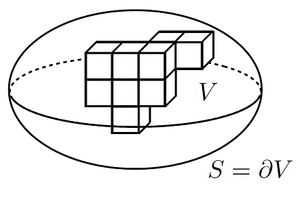
Fig. 7.4 Infinitesimal cubic volumes \(\mathrm{d}V = \mathrm{d}x\,\mathrm{d}y\,\mathrm{d}z\) breaking up a volume \(V\).

This means we are summing up neighbouring cubes, where the outgoing flux \(\int \,\mathrm{d}J > 0\) from one cube becomes an ingoing flux \(\int \,\mathrm{d}J < 0\) for an adjacent cube, as depicted in Fig. 7.5.

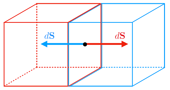
Fig. 7.5 A schematic of the infinitesimal flux contributions from neighbouring infintesimal cubic volumes.

Therefore we see that the only remaining contributions to the summing of the fluxes over the volume will be from the volumes surface, hence:

\[\int \mathrm{d}F = \iint_{S = \partial V}\,\mathrm{d}F = \iint_{\partial V}\,{\bf F}({\bf r})\cdot \mathrm{d}{\bf A} = \iiint_V \Bigg( \nabla \cdot {\bf G}({\bf r})\Bigg)\,\mathrm{d}V\]

which is the desired result.

7.3. (Kelvin-)Stoke’s Theorem

Definition

Stokes’s theorem states that for the curl of a vector field \({\bf F}({\bf r})\) over a surface \(S\) should match the line integral of the field over some closed contour \(C = \partial S\) around the boundary of \(S\):

\[\oint_{\partial S} {\bf F}({\bf r}) \cdot \mathrm{d}{\bf r} = \iint_{S} \Bigg(\nabla \times {\bf F}\Bigg)\cdot\mathrm{d}{\bf A}\]

where the orientation of this closed contour should match the direction of the surface normal, as given by the right hand rule depicted in Fig. 7.6.

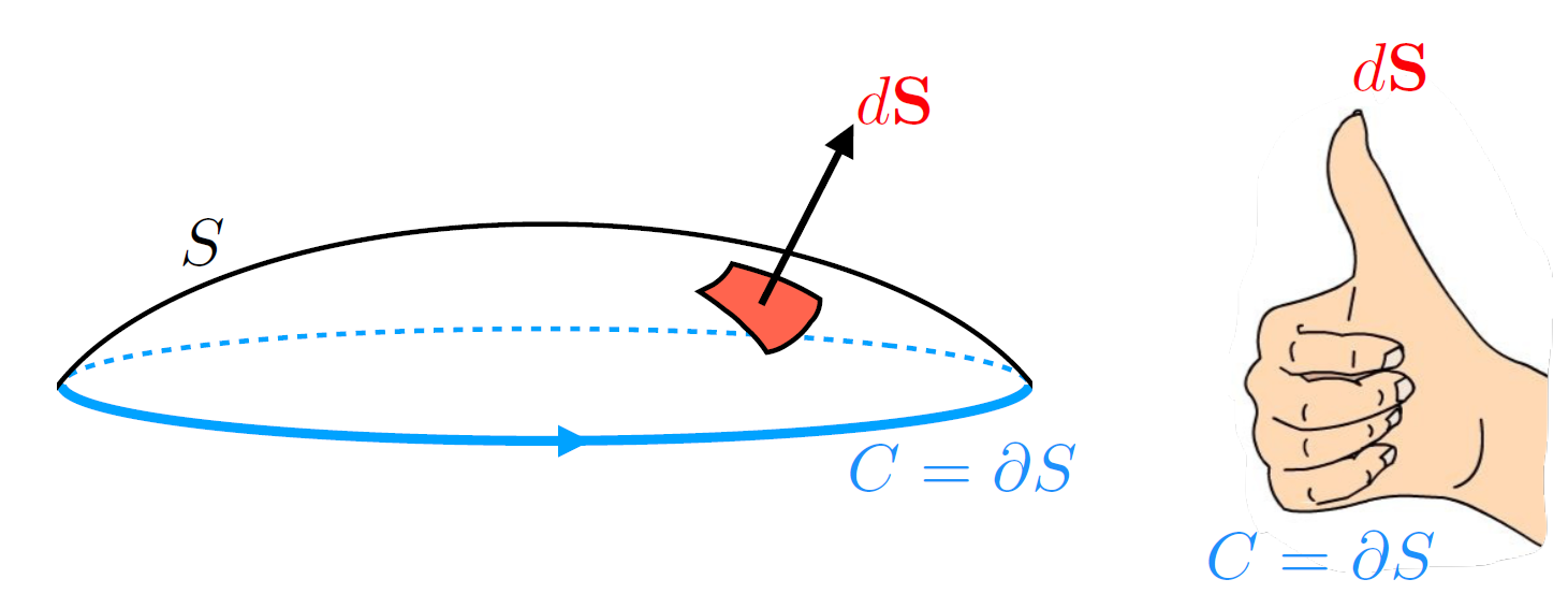
Fig. 7.6 The relevant orientation of the closed contour used in Stoke’s theorem using the right hand rule.

Worked example

Find the line integral of the vector field \({\bf F}({\bf r}) = \begin{pmatrix} y \\ -z \\ -x^2 \end{pmatrix}\) over a closed path, from \((0,\,0,\,0) \rightarrow (0,\, 1,\, 0)\), then along a circular arc of radius 1 to \((0,\,0,\,1)\) before going back to the origin. We depict this system in Fig. 7.7.

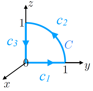
Fig. 7.7 Closed contour \(\mathcal{C}\) around the origin - we note that this contour bounds an area that is the quarter of a unit circle centered on the origin.

The parameterisation of the contours here will not change its result (nor should the starting point for a loop integral), so we will start at the origin and parameterise the three sections of the contour \(C_1,\,C_2,\, C_3\) using \(0 \leq t \leq 1\):

\[\begin{split}\mathcal{C}_1: {\bf r}(t) &= \begin{pmatrix} 0 \\ t \\ 0 \end{pmatrix} \Rightarrow {\bf F}({\bf r}) = \begin{pmatrix} t \\ 0 \\ 0 \end{pmatrix}, \quad {\bf r'}(t) = \begin{pmatrix} 1 \\ 0 \\ 0 \end{pmatrix}\\ \mathcal{C}_2: {\bf r}(t) &= \begin{pmatrix} 0 \\ \cos(\pi t/2) \\ \sin(\pi t/2) \end{pmatrix} \Rightarrow {\bf F}({\bf r}) = \begin{pmatrix} \cos(\pi t/2) \\ -\sin(\pi t/2) \\ 0 \end{pmatrix}, \quad {\bf r'}(t) = \begin{pmatrix} 0 \\ -\frac{\pi}{2}\sin(\pi t/2) \\ \frac{\pi}{2}\cos(\pi t/2) \end{pmatrix}\\ \mathcal{C}_3: {\bf r}(t) &= \begin{pmatrix} 0 \\ 0 \\ 1-t \end{pmatrix} \Rightarrow {\bf F}({\bf r}) = \begin{pmatrix} 0 \\ -(1-t) \\ 0 \end{pmatrix}, \quad {\bf r'}(t) = \begin{pmatrix} 0 \\ 0 \\ -1 \end{pmatrix}\end{split}\]

Therefore we can calculate the line integral:

\[\begin{split}& \int_C {\bf F}({\bf r})\cdot \mathrm{d}{\bf r} = \int_0^1 {\bf F}({\bf r})\cdot {\bf r'}\,\mathrm{d}t\\ &= \int_0^1 \left[ \begin{pmatrix} t \\ 0 \\ 0 \end{pmatrix} \cdot \begin{pmatrix} 0 \\ 1 \\ 0 \end{pmatrix} + \begin{pmatrix} \cos(\pi t/2) \\ -\sin(\pi t/2) \\ 0 \end{pmatrix}\cdot \begin{pmatrix} 0 \\ -\frac{\pi}{2}\sin(\pi t/2) \\ \frac{\pi}{2}\cos(\pi t/2) \end{pmatrix} + \begin{pmatrix} 0 \\ -(1-t) \\ 0 \end{pmatrix} \cdot\begin{pmatrix} 0 \\ 0 \\ -1 \end{pmatrix}\right]\,\mathrm{d}t\\ &= \frac{\pi}{2}\int_0^1\sin^2(\pi t/2)\,\mathrm{d}t = \frac{\pi}{4}\int_0^1\Bigg (1-\cos(\pi t)\Bigg)\,\mathrm{d}t = \frac{\pi}{4}\Bigg[t - \frac{1}{\pi}\sin(\pi t)\Bigg]_0^1 =\frac{\pi}{4}\end{split}\]

Using Stoke’s theorem, we are free to find formally any surface which would be bounded by the contour - however clearly the easiest to work with is the area of the quarter circle, sitting on the \(y-z\) plane. To make sure the orientation of the contour matches with the right hand rule, we have:

\[\mathrm{d}{\bf A} = \mathrm{d}y\,\mathrm{d}z\,\hat{\bf x} \]

Therefore given that we can find the cross product as:

\[\begin{split}\nabla \times {\bf F} = \begin{vmatrix} \hat{\bf x} & \hat{\bf y} & \hat{\bf z} \\ \partial_x & \partial_y & \partial _ z \\ y & -z & -x^2\end{vmatrix} = \begin{pmatrix} \partial_y(-x^2) - \partial_z(-z) \\ \partial_z(y) - \partial_x(-x^2) \\ \partial_x(-z) - \partial_y(y) \end{pmatrix} = \begin{pmatrix} 1\\ 2x\\ -1\end{pmatrix}\end{split}\]

we can find:

\[\begin{split}& \iint_S\Bigg( \nabla \times {\bf F}\Bigg)\cdot\mathrm{d}{\bf A} = \iint_S \begin{pmatrix} 1\\ 2x\\ -1\end{pmatrix}\cdot \begin{pmatrix} 1\\ 0\\ 0\end{pmatrix}\,\mathrm{d}y\,\mathrm{d}z\\ &= \iint_S \,\mathrm{d}y\,\mathrm{d}z = \frac{1}{4}\left(\pi 1^2\right) = \frac{\pi}{4}\end{split}\]

Therefore for quite a lot less work, we find the same result!

7.3.1. A Sketch of a Proof

Lets consider a vectorial surface area element \(\mathrm{d}{\bf A} = \mathrm{d}x\,\mathrm{d}y\,\hat{\bf z}\), as depicted in Fig. 7.8:

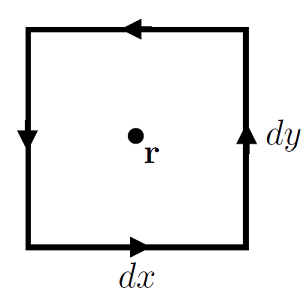
Fig. 7.8 Closed infinitesimal contour around some point \({\bf r}\).

We can find the an infinitesimal loop \(\mathrm{d}\ell\) of a vector field \({\bf F}({\bf r})\) around this contour as:

\[\begin{split}\mathrm{d}\ell &= {\bf F}\left({\bf r} - \frac{1}{2}\mathrm{d}y\,\hat{\bf y} \right)\cdot \hat{\bf x}\,\mathrm{d}x + {\bf F}\left({\bf r} + \frac{1}{2}\mathrm{d}x\,\hat{\bf x} \right)\cdot \hat{\bf y}\,\mathrm{d}y \\ &+\, {\bf F}\left({\bf r} + \frac{1}{2}\mathrm{d}y\,\hat{\bf y} \right)\cdot (-\hat{\bf x})\,\mathrm{d}x + {\bf F}\left({\bf r} - \frac{1}{2}\mathrm{d}x\,\hat{\bf x} \right)\cdot (-\hat{\bf y})\,\mathrm{d}y \\ &= \left[F_x \left({\bf r} - \frac{1}{2}\mathrm{d}y\,\hat{\bf y} \right) - F_x\left({\bf r} + \frac{1}{2}\mathrm{d}y\,\hat{\bf y} \right) \right]\,\mathrm{d}x + \left[ F_y\left({\bf r} + \frac{1}{2}\mathrm{d}x\,\hat{\bf x} \right) - F_y\left({\bf r} - \frac{1}{2}\mathrm{d}x\,\hat{\bf x} \right)\right]\,\mathrm{d}y\end{split}\]

If we do a Taylor expansion of each vector field, around \(F_x({\bf r})\):

\[\begin{split}\mathrm{d}\ell &= \left[F_x({\bf r}) - \frac{1}{2}\partial_y F_x({\bf r})\,\mathrm{d}y - \left(F_x({\bf r}) + \frac{1}{2}\partial_y F_x({\bf r})\,\mathrm{d}y \right)\right]\,\mathrm{d}x\\ &+ \left[F_y({\bf r}) + \frac{1}{2}\partial_x F_y({\bf r})\,\mathrm{d}x - \left(F_y({\bf r}) = \frac{1}{2}\partial_x F_y({\bf r})\,\mathrm{d}x \right)\right]\,\mathrm{d}y\\ &= -\partial_y F_x({\bf r})\,\mathrm{d}x\,\mathrm{d}y + \partial_x F_y({\bf r})\,\mathrm{d}x\,\mathrm{d}y \end{split}\]

We can read this last expression as the \(z\) component of the curl of \({\bf F}({\bf r})\):

\[\mathrm{d}\ell = \Bigg(\nabla \times {\bf G}\Bigg)_z\,\mathrm{d}x\,\mathrm{d}y\]

So this is really just a dot product with the \(z\) vector:

\[\begin{split}\mathrm{d}\ell &= \Bigg(\nabla \times {\bf G}\Bigg)\cdot \hat{\bf z}\,\mathrm{d}x\,\mathrm{d}y \\ &= \Bigg(\nabla \times {\bf G}\Bigg)\cdot\mathrm{d}{\bf S}\end{split}\]

where we have taken this second part as the area vector normal \(\mathrm{d}{\bf A}\) to the \(x-y\) plane.

We can integrate this expression up to find:

\[\ell = \iint_S (\nabla \times {\bf F})\cdot \mathrm{d}{\bf A}\]

Thinking carefully these loop integrals however, if we sum up infinitesimal areas (plaquettes if you will), then only the plaquettes on the surface will not have have cancellation occuring, as depicted in Fig. 7.9:

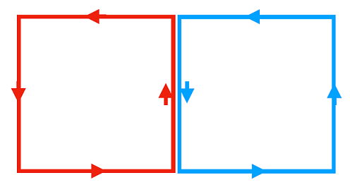
Fig. 7.9 Neighbouring infinitesimal contours along some surface, we find that there will be a net cancellation occuring along shared sides.

and hence:

\[\int_S\,\mathrm{d}\ell = \oint_{\partial S}{\bf F}\cdot \mathrm{d}{\bf r} = \iint_S (\nabla \times {\bf F})\cdot \mathrm{d}{\bf A}\]

which is the desired result.

7.4. Green’s Theorem

Definition

Green’s theorem states that in two dimensional systems, the following relation holds:

\[\int_{\partial S} \left[L(x,\,y)\,\mathrm{d}x + M(x,\,y)\,\mathrm{d}y\right] = \iint_S \left(\frac{\partial M}{\partial x} - \frac{\partial L}{\partial y} \right)\,\mathrm{d}x\,\mathrm{d}y\]

where \(\partial S\) is a boundary defined in the anti-clockwise orentiation around surface \(S\).

Green’s theorem is really just Stoke’s theorem in 2D, which allows for a simpler expression of the formulae.

Consider a vector field defined in the \(x-y\) plane:

\[\begin{split}{\bf F} = \begin{pmatrix} F_x \\ F_y \\ 0\end{pmatrix}\end{split}\]

the curl of this will be found to be:

\[\begin{split}\nabla \times {\bf F} = \begin{vmatrix} \hat{\bf x} & \hat{\bf y} & \hat{\bf z} \\ \partial_x & \partial_y & \partial_z \\ F_x & F_y & 0\end{vmatrix} = \begin{pmatrix} \partial_y(0) - \partial_x(F_y) \\ \partial_z(F_x) - \partial_x(0) \\ \partial_x(F_y) - \partial_y(F_x) \end{pmatrix} \end{split}\]

Given Stoke’s theorem:

\[\oint_{\partial S} {\bf F}\cdot\mathrm{d}{\bf r} = \iint_S (\nabla \times {\bf F})\cdot \mathrm{d}{\bf A}\]

and the fact that the surface normal area must be of the form:

\[\mathrm{d}{\bf A} = \hat{\bf z}\,\mathrm{d}x\,\mathrm{d}y\]

along with the line integral here being of the form:

\[{\bf F} \cdot \mathrm{d}{\bf r} = F_x\,\mathrm{d}x + F_y\,\mathrm{d}y\]

IF the boundary of \(S\) is defined in the anti-clockwise orentiation. Putting these together:

\[\int_{\partial S} \left[F_x\,\mathrm{d}x + F_y\,\mathrm{d}y\right] = \iint_S \left(\frac{\partial F_y}{\partial x} - \frac{\partial F_x}{\partial y} \right)\,\mathrm{d}x,\,\mathrm{d}y\]