4.3. Workshop 4: Modelling Space#
We’ve already seen that we can use arrays to store one-dimensional sequences of numerical data. Such data might represent a time series of measurements, such as daily recordings of atmospheric pressure (Fig. 4.3) where the value x[i] in the array x corresponds to the pressure on day i.
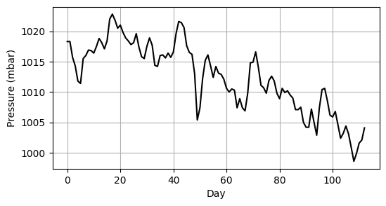
Fig. 4.3 Atmospheric pressure measured for 113 consecutive days.#
On the other hand, we might need to work with data that is two-dimensional, such as recordings of atmospheric pressure over a rectangular region. The values in the array are then indexed by two numbers so that x[i, j] corresponds to the pressure at the coordinate i, j. Such arrays can be represented as a heat map, which is an image where the intensity of each pixel represents the value of the array element (Fig. 4.4).
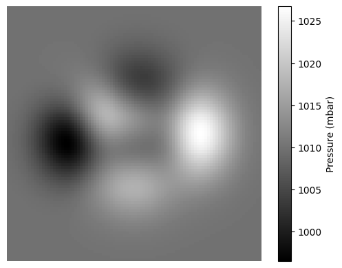
Fig. 4.4 Atmospheric pressure over a 2d rectangular area.#
1D Moving Average#
A moving average is commonly used when visualising time series data in order to smooth out short-term fluctuations in the data. Fig. 4.5 shows 113 days of atmospheric pressure along with the 10-day and 5-day moving averages.
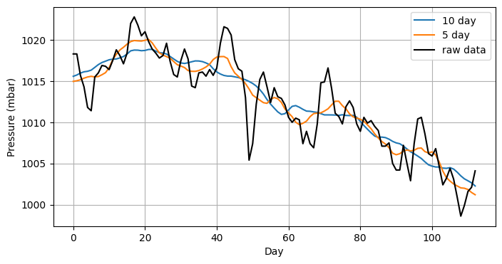
Fig. 4.5 Atmospheric pressure measured for 113 consecutive days, along with 10-day and 5-day moving averages, where the \(k\)-day moving averages are taken over \(2k+1\) measurements centred at each day.#
In this workshop, we define the k-moving average of an array as the array formed by averaging \(k\) values on either side of each element (a total of \(2k + 1\) elements). For example, given a sequence of values \(x_i\) then the 1-moving average \(y_i\) is defined by (see Fig. 4.6):
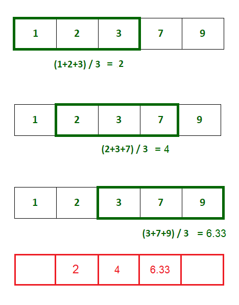
Fig. 4.6 Calculate the 1-moving average of an array as the mean of consecutive triples.#
We can calculate the 1-moving average in Python as follows.
import numpy as np

x = np.array([1.0, 5.0, 3.4, 2.1, 6.5, 2.4, 3.1])
n = len(x)

y = np.zeros(n)

for i in range(1, n - 1):
    y[i] = (x[i-1] + x[i] + x[i+1]) / 3

print("1-moving average:", y)
1-moving average: [0.         3.13333333 3.5        4.         3.66666667 4.
 0.        ]
A more compact way to calculate the sum of consecutive elements is using numpy slice notation. We can replace (x[i-1] + x[i] + x[i+1])/3 with np.average(x[i-1:i+2]). x[a:b] represents the subarray from a to b (including the lower limit but excluding the upper limit).
y = np.zeros(n)
for i in range(1, n - 1):
    y[i] = np.average(x[i-1:i+2])

print("1-moving average:", y)
1-moving average: [0.         3.13333333 3.5        4.         3.66666667 4.
 0.        ]
Notice that when i=0 or i=n the subarray x[i-1:i+2] would include elements outside the bounds of the array x. The for loop therefore excludes the first and last element in its range function and we end up with zeros padding the start and end of the array.
Exercise 4.5
Calculate the 2-moving average of x. You should get the following result:
[0. 0. 3.6 3.88 3.5 0. 0. ]
Exercise 4.6
Write a function moving_average(x, k) which returns an array containing the k-moving average of x.
def moving_average(x, k):
    n = len(x)
    y = np.zeros(n)

    # your code

    return y
Check that moving_average(x, 1) and moving_average(x, 2) produce the correct 1- and 2-moving averages, as previously calculated.
Instead of padding the start and end of the array with zeros, we can simply average only the elements of the subarray x[i-1:i+2] which lie within the bounds of x. In the case of the 1-moving average we can achieve this by replacing the lower limit with max(i-1, 0) and the upper limit with min(i+2, n). We also change the for loop to include the full range from 0 to n.
y = np.zeros(n)
for i in range(0, n):
    y[i] = np.average(x[max(i-1,0):min(i+2, n)])

print("1-moving average:", y)
1-moving average: [3.         3.13333333 3.5        4.         3.66666667 4.
 2.75      ]
Exercise 4.7
Change your function moving_average(x, k) to remove the zero-padding.
The array pressure_data contains the atmospheric pressure (measured in millibars) shown in Fig. 4.3.
pressure_data = [1018.3, 1018.3, 1015.7, 1014.3, 1011.8, 1011.4, 1015.5, 1016.0, 1016.9, 1016.8, 1016.4, 1017.5, 1018.8, 1018.1, 1017.1, 1018.4, 1022.0, 1022.8, 1021.8, 1020.5, 1021.0, 1019.8, 1018.9, 1018.4, 1017.8, 1018.1, 1019.6, 1017.4, 1015.8, 1015.5, 1017.5, 1018.9, 1017.7, 1014.4, 1014.2, 1016.0, 1016.1, 1015.6, 1016.4, 1015.7, 1016.6, 1019.6, 1021.6, 1021.4, 1020.6, 1017.6, 1016.5, 1016.2, 1013.0, 1005.4, 1007.4, 1012.2, 1015.2, 1016.1, 1014.3, 1012.4, 1014.2, 1013.1, 1012.9, 1012.1, 1010.6, 1010.0, 1010.5, 1010.3, 1007.4, 1008.9, 1007.4, 1006.9, 1009.8, 1014.8, 1014.9, 1016.6, 1014.1, 1011.1, 1010.7, 1009.8, 1011.9, 1012.6, 1011.8, 1009.8, 1008.9, 1010.6, 1009.9, 1010.2, 1009.5, 1009.0, 1007.1, 1007.1, 1007.5, 1005.0, 1004.2, 1004.2, 1007.2, 1005.0, 1002.9, 1007.4, 1010.4, 1010.6, 1008.6, 1006.2, 1005.9, 1006.8, 1004.6, 1002.4, 1003.2, 1004.4, 1003.1, 1000.9, 998.6, 999.9, 1001.6, 1002.1, 1004.1]
Exercise 4.8
Plot the atmospheric pressure data on a line graph. On the same graph, plot the 5- and 10-moving averages (as shown in Fig. 4.5).
2D Moving Average#
We can extend the definition of moving average to 2-dimensional data. One application of moving averages on 2-dimensional data is smoothing images. In Fig. 4.7 the image on the left is an n by m array where the colour intensity of each pixel corresponds to the value of each array element. Applying a 2-dimensional moving average to each pixel result in the smoothed image on the right.
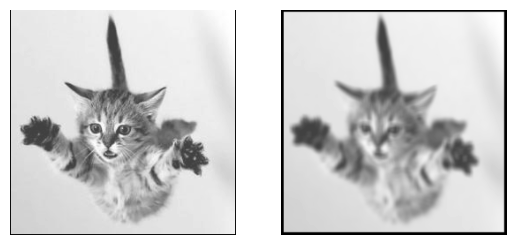
Fig. 4.7 An image before (left) and after (right) 2-dimensional averaging.#
The 2-dimensional 1-moving average is calculated by taking the average of the 9 values in the 3 by 3 sub-array centred at each element (see figure Fig. 4.8). In the example below we do this calculation for a single cell x[1,1] of a 5 by 5 array x.
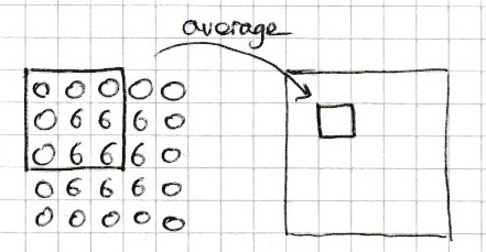
Fig. 4.8 The 1-moving average of the cell at position 1, 1 is the average of the 9 surrounding cells.#
import numpy as np
import matplotlib.pyplot as plt

x = np.array([[0, 0, 0, 0, 0],
              [0, 6, 6, 6, 0],
              [0, 6, 6, 6, 0],
              [0, 6, 6, 6, 0],
              [0, 0, 0, 0, 0]])

# calculate the 2d moving average of the cell x[1, 1]
sub_array = x[0:3, 0:3]
average = np.average(sub_array)

print("3 by 3 sub array:\n", sub_array)
print("average:", average)
3 by 3 sub array:
 [[0 0 0]
 [0 6 6]
 [0 6 6]]
average: 2.6666666666666665
Then we can then create a second array to store the result:
y = np.zeros((5, 5))

y[1, 1] = average

print(y)
[[0.         0.         0.         0.         0.        ]
 [0.         2.66666667 0.         0.         0.        ]
 [0.         0.         0.         0.         0.        ]
 [0.         0.         0.         0.         0.        ]
 [0.         0.         0.         0.         0.        ]]
Exercise 4.9
Complete the following code to calculate the 2d 1-moving average for all cells in x (except the cells along each edge).
x = np.array([[0, 0, 0, 0, 0],
              [0, 6, 6, 6, 0],
              [0, 6, 6, 6, 0],
              [0, 6, 6, 6, 0],
              [0, 0, 0, 0, 0]])

y = np.zeros((5, 5))

for i in range(1, 4):
    for j in range(1, 4):
        # calculate the average of the 3 by 3
        # subarray centred at cell i, j
        # then store in the appropriate cell of y
Check you get the correct answer as below.
print(y)
[[0.         0.         0.         0.         0.        ]
 [0.         2.66666667 4.         2.66666667 0.        ]
 [0.         4.         6.         4.         0.        ]
 [0.         2.66666667 4.         2.66666667 0.        ]
 [0.         0.         0.         0.         0.        ]]
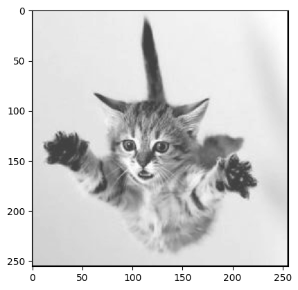
Now let’s try this procedure on the image shown in Fig. 4.7. The data for this image can be found in the file falling_cat.txt. The following code can be used to load the image file into a numpy array, then display the contents of the array.
x = np.loadtxt("falling_cat.txt")
plt.imshow(x, cmap="gray")
<matplotlib.image.AxesImage at 0x1aeb4329e08>
Exercise 4.10
Load the file falling_cat.txt into a numpy array. Use your code from the previous question to calculate its 1-moving average, then use plt.imshow to display the image before and after smoothing. You should end up with two images similar to Fig. 4.7.
Hint: you can use x.shape to find the dimensions of the original array.
x = np.loadtxt("falling_cat.txt")
plt.imshow(x, cmap="gray")
n, m = x.shape
y = np.zeros((n, m))
The 2-dimensional 1-moving average calculates the average across 3 by 3 subarrays centred at each array element. Similarly, we can calculate the k-moving average across \(2k+1\) by \(2k+1\) subarrays.
Exercise 4.11
Adapt your code so that it calculates the k-moving average of the array x.
Then, write a function moving_average_2d(x, k) which returns the k-moving average of the 2d array x. Test your function against the cat image for various values of k. Bigger values of k should result in a more blurry image.
def moving_average_2d(x, k):
    # your code here

x = np.loadtxt("falling_cat.txt")
plt.figure()
plt.imshow(x, cmap="gray")


# this should result in a very blurry image
y = moving_average_2d(x, 8)
plt.figure()
plt.imshow(y, cmap="gray")