Solutions

Solution to Exercise 3.6

In order to decide how to calculate the next term in the sequence, we need to work out whether \(n\) is even or odd. Recall from tutorial 1 that we can use the modulus operator % to find the remainder after floor division. So if \(n % 2\) is equal to \(0\) then \(n\) must be even.

def collatz_op(n):
    if (n % 2) == 0:     # check if n is even
        next_term = n / 2
    else:                # must be odd
        next_term = (n * 3) + 1 
    
    return next_term

We can check the function works by trying it out for n = 5 and n = 6. When n = 5 we triple it and add 1, so the next term if 16. When n = 6 we divide it by two so the next term is 3.

print(collatz_op(5))
print(collatz_op(6))

16
3.0

Solution to Exercise 3.7

To calculate the Collatz Number of n we need to iteratively calculate the next term in the sequence until we get to 1 and calculate how many iterations we used. Note that the Collatz Number of 1 is 1, so the counter should be initialised to 1.

def collatz_number(n):
    num = 1
    while n > 1:
        num += 1
        n = collatz_op(n)
    
    return num

Let’s check this works using n = 5 and n = 6. We know that the Collatz Number of \(5\) is \(6\). When \(n\) is \(6\), the Collatz Sequence is \(6, 3, 10, 5, 16, 8, 4, 2, 1\) so the Collatz Number is \(9\).

print('The Collatz Number of 5 is ', collatz_number(5))
print('The Collatz Number of 6 is ', collatz_number(6))

The Collatz Number of 5 is  6
The Collatz Number of 6 is  9

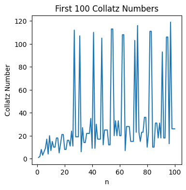
Solution to Exercise 3.8

import numpy as np
import matplotlib.pyplot as plt

collatz_numbers = np.zeros(100)

for i in range(100):
    collatz_numbers[i] = collatz_number(i + 1)

# remember to plot the collatz numbers against 1-100, not 0-99
plt.figure(figsize=(4,4))
plt.plot(np.linspace(1, 100, 100), collatz_numbers)
plt.title('First 100 Collatz Numbers')
plt.xlabel('n')
plt.ylabel('Collatz Number')

Text(0, 0.5, 'Collatz Number')

Solution to Exercise 3.9

Using our code from last week, we just need to make a little addition to calculate peak infections:

import numpy as np
import matplotlib.pyplot as plt

# set up variables and arrays
n_days = 100
a = 0.1
b = 0.00005
S = np.zeros(n_days)
I = np.zeros(n_days)

# initialise the variables
S[0] = 20000
I[0] = 100

# implement equations
for i in range(n_days - 1):
    S[i+1] = S[i] - (b * S[i] * I[i])
    I[i+1] = I[i] + (b * S[i] * I[i]) - (a * I[i])

# plot the figure
plt.figure(figsize=(5,5))
plt.plot(I)
plt.plot(S)
plt.xlabel("Time (days)")
plt.ylabel("Population")


# check the maximum 
peak_infections = np.max(I)
print('For infection rate', b, 'infections peak at', peak_infections, 'cases.')

For infection rate 5e-05 infections peak at 14873.5610390745 cases.

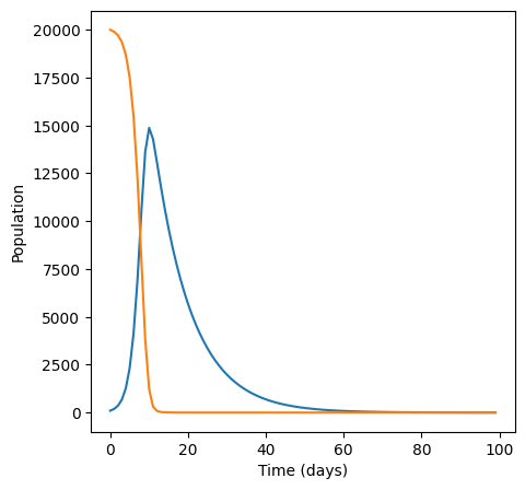
Looking at the graph, infections peak at around \(15000\) cases, which is similar to what we find frpom np.max. Let’s check for another value of \(b\).

import numpy as np
import matplotlib.pyplot as plt

# set up variables and arrays
n_days = 100
a = 0.1
b = 0.00001
S = np.zeros(n_days)
I = np.zeros(n_days)

# initialise the variables
S[0] = 20000
I[0] = 100

# implement equations
for i in range(n_days - 1):
    S[i+1] = S[i] - (b * S[i] * I[i])
    I[i+1] = I[i] + (b * S[i] * I[i]) - (a * I[i])

# plot the figure
plt.figure(figsize=(5,5))
plt.plot(I)
plt.plot(S)
plt.xlabel("Time (days)")
plt.ylabel("Population")


# check the maximum 
peak_infections = np.max(I)
print('For infection rate', b, 'infections peak at', peak_infections, 'cases.')

For infection rate 1e-05 infections peak at 3245.641623687537 cases.

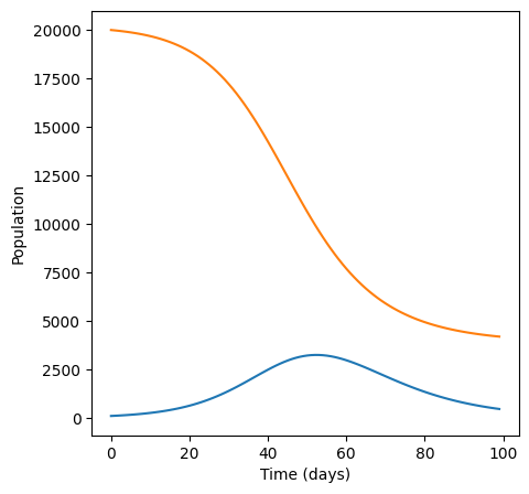
This time, both from np.max and by visually inspecting the graph we see that the peak number of infections is much lower.

Solution to Exercise 3.10

1. First we need to write a function that will return the maximum number of infected people for different parameter values. We can just modify the code above so that it is inside a function:

def max_infected(a, b):
    # Run the simulation and calculate
    # the peak number of infections
    
    # set up variables and arrays
    n_days = 100
    S = np.zeros(n_days)
    I = np.zeros(n_days)

    # initialise the variables
    S[0] = 20000
    I[0] = 100

    # implement equations
    for i in range(n_days - 1):
        S[i+1] = S[i] - (b * S[i] * I[i])
        I[i+1] = I[i] + (b * S[i] * I[i]) - (a * I[i])
        
    # check the maximum 
    peak_infections = np.max(I)
    
    return peak_infections

We can check this works by calling the function for a = 0.1 and the values of b we tested above. For example:

max_infected(0.1, 0.00005)

14873.5610390745

returns \(14873\), as we expect!

2. Recall from last week that to generate 10 evenly spaced numbers from 0 to 0.00005 we can use:

b_array = np.linspace(0, 0.00005, 10)

3. Again, recall from last week that we can create an array containing 10 zeros:

peak_infections = np.zeros(10)

4. We have also seem how to use a loop to set a value in an array - notice that we need to retrieve each value of b to test from b_array.

for i in range(10):
    # Calculate the peak number of infections
    # for the given value of b
    peak_infections[i] = max_infected(0.1, b_array[i])

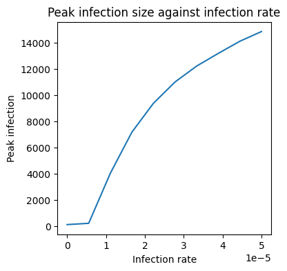
5. Now we just need to plot the peak_infections array against b_array to see how peak infections vary with the infection parameter.

# Create a plot of peak infections against b
plt.figure(figsize=(4,4))
plt.plot(b_array, peak_infections)
plt.title('Peak infection size against infection rate')
plt.xlabel('Infection rate')
plt.ylabel('Peak infection')

Text(0, 0.5, 'Peak infection')

Putting this altogether we have:

def max_infected(a, b):
    # Run the simulation and calculate
    # the peak number of infections
    
    # set up variables and arrays
    n_days = 100
    S = np.zeros(n_days)
    I = np.zeros(n_days)

    # initialise the variables
    S[0] = 20000
    I[0] = 100

    # implement equations
    for i in range(n_days - 1):
        S[i+1] = S[i] - (b * S[i] * I[i])
        I[i+1] = I[i] + (b * S[i] * I[i]) - (a * I[i])
        
    # check the maximum 
    peak_infections = np.max(I)
    
    return peak_infections

b_array = np.linspace(0, 0.00005, 10)
peak_infections = np.zeros(10)

for i in range(10):
    # Calculate the peak number of infections
    # for the given value of b
    peak_infections[i] = max_infected(0.1, b_array[i])

# Create a plot of peak infections against b
plt.figure(figsize=(4,4))
plt.plot(b_array, peak_infections)
plt.title('Peak infection size against infection rate')
plt.xlabel('Infection rate')
plt.ylabel('Peak infection')

Text(0, 0.5, 'Peak infection')

As we expect, as the infection rate grows so does the peak infection!

Solution to Exercise 3.11

We can use the function np.sum to sum the values in an array. To find out the total number of infected person-days we just need to sum the values in I - so we just need to make a small tweak to the max_infected function we wrote above:

def total_infected(a, b):
    # Run the simulation and calculate
    # the total number of infections

    # set up variables and arrays
    n_days = 100
    S = np.zeros(n_days)
    I = np.zeros(n_days)

    # initialise the variables
    S[0] = 20000
    I[0] = 100

    # implement equations
    for i in range(n_days - 1):
        S[i+1] = S[i] - (b * S[i] * I[i])
        I[i+1] = I[i] + (b * S[i] * I[i]) - (a * I[i])

    # check the total - sum instead of max!
    total_infections = np.sum(I)

    return total_infections

This code is tricky to test as it is not easy to see the total infected person-days from the graph! However, when \(b = 0\) and \(a = 1\), the equations reduce to

(3.2)\[\begin{split}\begin{align}S_{i+1} &= S_i \\ I_{i+1} &= 0.\end{align}\end{split}\]

so everyone recovers after just \(1\) day, and no one else is infected. This means the total infected person-days for these parameter values should be \(100\) - let’s check!

total_infected(1, 0)

100.0

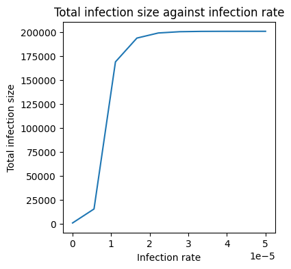
Now we just need to plot the total infected person-days for different values of \(b\) - just like we did above:

# set up variables and arrays
b_array = np.linspace(0, 0.00005, 10)
total_infections = np.zeros(10)

for i in range(10):
    # Calculate the total number of infections
    # for the given value of b
    total_infections[i] = total_infected(0.1, b_array[i])

# Create a plot of total infections against b
plt.figure(figsize=(4,4))
plt.plot(b_array, total_infections)
plt.title('Total infection size against infection rate')
plt.xlabel('Infection rate')
plt.ylabel('Total infection size')

Text(0, 0.5, 'Total infection size')

Solution to Exercise 3.12

As above, let’s check the costs for 10 values of \(b\) in the range \(0\) to \(0.00005\). We need to set up arrays to contain the costs and then calculate the corresponding cost for each value of \(b\).

Notice that when \(b = 0\) the formula suggests the intervention cost will be infinite - Python cannot handle dividing by zero (try it!) and will throw an error. To get around this, we can use np.linspace to set up the array for \(b\) as normal, and then just make the first element non-zero (but still small).

Also notice that rather than initialising a third array and calculating each element of total_cost one by one, we have just been able to add the intervention_cost and medical_cost arrays together - this works because they are both the same size!

# set up variables and arrays
b_array = np.linspace(0, 0.00005, 10)
intervention_cost = np.zeros(10)
medical_cost = np.zeros(10)

# avoid b = 0
b_array[0] = 0.000001

for i in range(10):
    intervention_cost[i] = 1/(5 * b_array[i]) - 2000
    medical_cost[i] = total_infected(0.1, b_array[i])

# add up the total cost
total_cost = intervention_cost + medical_cost

# Create a plot of costs against b
plt.figure(figsize=(4,4))
plt.plot(b_array, intervention_cost)
plt.plot(b_array, medical_cost)
plt.plot(b_array, total_cost)
plt.title('Costs against infection rate')
plt.xlabel('Infection rate')
plt.ylabel('Cost (thousands of £s)')

Text(0, 0.5, 'Cost (thousands of £s)')

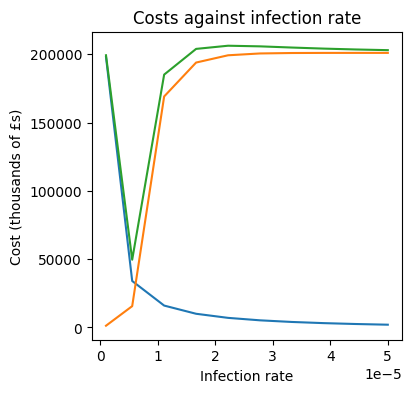
Examining the graph, we can see that costs are minimised when \(b \approx 5 \times 10^{-6}\).